Objective 3. Use COUNTIF and IF Functions, and Apply Conditional Formatting
Statistical functions analyze a group of measurements. Logical functions test for specific conditions; logical functions commonly use conditional tests to determine whether specified conditionscalled criteriaare true or false.
Activity 3.5. Rotating Text in a Cell
The worksheet that you will use to confirm if the management guideline is met indicates the time slots as column headings. One way to format long column titles is to wrap the text in the cell. Another way to format long column titles is to rotate the text within the cell.
|
1. |
Start the Excel program. Click Open |
|
2. |
In the Name Box, type b2:q2 and press |
|
3. |
Under Orientation, in the Degrees box type 45 to increase the orientation to 45 and then compare your screen with Figure 3.15. Figure 3.15. 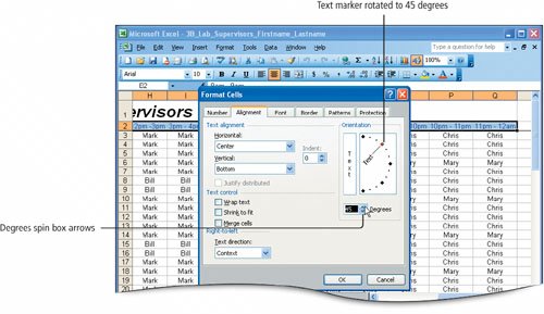
Alternatively, under Orientation, drag the red box at the end of the Text marker to the desired angle, or click the Degrees spin box up arrow. |
|
|
|
|
4. |
In the Format Cells dialog box, click OK to display the text at a 45-degree angle. Select the range A2:Q2, display the Format Cells dialog box, and then click the Border tab. Under Presets, click Inside, and then click OK. |
|
5. |
In the Name Box, type a:q and press Figure 3.16. 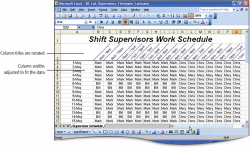
The selected column widths are adjusted to fit the width of the contents, which makes the data range narrower. This technique is useful when the column titles are wider than the data in the columns. |
 , navigate to the folder where the student files for this textbook are stored, and then open e03B_Lab_Supervisors. Display the Save As dialog box, navigate to your Excel Chapter 3 folder, and then save the workbook as 3B_Lab_Supervisors_Firstname_Lastname
 to select the column headings. From the Format menu, display the Format Cells dialog box, and then click the Alignment tab.
 your workbook, and then compare your screen with Figure 3.16.
Activity 3.6. Using the COUNTIF Function
The COUNTIF function counts the number of cells within a range that meet the given conditionthe criteria that you provide. The COUNTIF function has two argumentsthe range of cells to check and the criteria.
|
1. |
Scroll to view rows 35:42 on your screen, and notice that as you scroll, rows 1 and 2 remain visible because the Freeze Panes command has been applied. |
|
2. |
Click cell B39. On the Formula Bar, click the Insert Function button |
|
|
|
|
3. |
Under Select a function, scroll down and click COUNTIF, and then click OK. In the displayed Function Arguments dialog box, in the Range box, type $b$3:$q$33 and then press |
|
4. |
In the Criteria box, type a39 and then compare your screen with Figure 3.17. Figure 3.17. 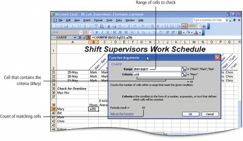
The formula will look at all the cells in the range and then count how many times the value in cell A39Maryoccurs. |
|
5. |
Click OK. |
|
6. |
With cell B39 as the active cell, drag the fill handle down through cell B42 to count the number of times that each supervisor's name occurs in the selected range, and then compare your screen with Figure 3.18. Figure 3.18. 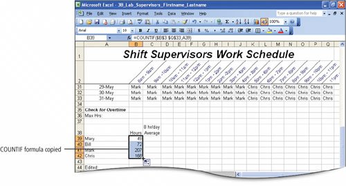
The occurrences of the other supervisor names are counted. By using the absolute reference to the range of cells and a relative reference to the first supervisor's name, the formula can be copied instead of rewritten each time. |
|
7. |
Click cell B40 and examine the formula. Notice that the range for the first argument$B$3:$Q$33did not change because of the absolute reference; but, the second argument for the criteria did change because of the relative cell reference. Click cell B41 and then B42 and examine the formula in each cell. |
|
8. |
Save |
 . In the displayed Insert Function dialog box, click the Or select a category arrow, and then click Statistical.
 . Alternatively, click the Collapse Dialog Box button, select the range b3:q33, press
  to apply the absolute cell reference, and then click the Expand Dialog Box button.
Activity 3.7. Using the If Function and Applying Conditional Formatting
A logical test is any value or expression that can be evaluated as being true or false. The IF function uses a logical test to check whether a condition is met, and then returns one value if true, and another value if false. For example, C8=100 is an expression that can be evaluated as true or false. If the value in cell C8 is equal to 100, the expression is true. If the value in cell C8 is not 100, the expression is false.
In this activity, you will use the IF function to determine whether any supervisor's proposed May schedule exceeds an average of 8 hours per day248 hours for the month.
|
1. |
Click cell B36. Type 248 and press |
||||||||||||||
|
|
|||||||||||||||
|
2. |
Click cell C39. Click the Insert Function button |
||||||||||||||
|
3. |
With the insertion point positioned in the Logical_test box, type b39<=$b$36 |
||||||||||||||
|
4. |
Take a moment to examine the table in Figure 3.19 for a list of logical operator symbols and their definitions.
|
||||||||||||||
|
5. |
Press |
||||||||||||||
|
6. |
Press Figure 3.20. (This item is displayed on page 806 in the print version) 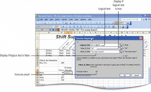
If the result of the logical test is falsethe number of hours worked is greater than 248then Excel will display Too many hours in the cell. |
||||||||||||||
|
|
|||||||||||||||
|
7. |
Click OK to display the result OK in cell C39. Using the fill handle, copy the formula down through cell C42. Save Figure 3.21. 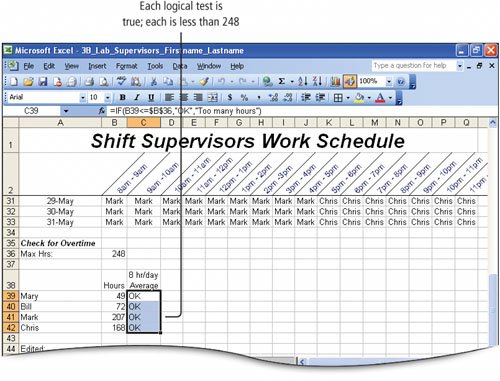
|
||||||||||||||
|
8. |
Click cell C40 and examine the formula. Notice that the first argument has been adjusted to examine cell B40 and compare it to $B$36. Click cell C41 and cell C42 to examine each formula to see that this pattern is followed. |
Activity 3.8. Applying Conditional Formatting
Conditional formatting is a format, such as cell shading or font color, that Excel applies to cells if a specified condition is true. Conditional formatting uses a dialog box to create the logical test, and then you choose the format to apply if the test is true. In this activity, you will use conditional formatting as another way to draw attention to the condition if one of the supervisors exceeds the maximum.
|
1. |
Select the range B39:B42, and then from the Format menu, click Conditional Formatting. |
|
2. |
In the displayed Conditional Formatting dialog box, under Condition 1, in the second box click the arrow, and then click greater than. |
|
3. |
Press Figure 3.22. (This item is displayed on page 808 in the print version) 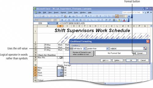
The special format that you specify will be applied to any cell in the selected range if its value is greater than the value in cell B36, which is 248. |
|
|
|
|
4. |
In the Conditional Formatting dialog box, click the Format button. In the displayed Format Cells dialog box, click the Font tab. Under Font style, click Bold. Click the Color arrow and in the third row, click the first colorRed. Compare your screen with Figure 3.23. Figure 3.23. 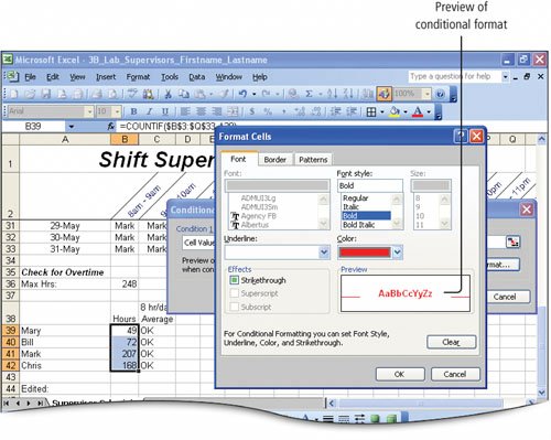
If the logical test is true, the content of the cell will be displayed in bold and in red, as displayed in the Preview box. |
|
5. |
In the Format Cells dialog box, click OK. In the Conditional Formatting dialog box, click OK. |
|
6. |
Click cell B36, type 100 and then press Figure 3.24. 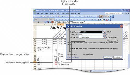
The Function Arguments dialog box displays the function arguments applied to cell C41. If B41 (207 hours) is less than or equal to B36 (100 hours), the result of the test condition is FALSE; therefore "Too many hours" displays in C41. |
|
|
|
|
7. |
Click Cancel to close the Function Arguments dialog box. Click cell B41, and then from the Format menu, click Conditional Formatting. |
|
8. |
Click Cancel to close the Conditional Formatting dialog box. In cell B36, type 248 and press |
Activity 3.9. Using Find and Replace to Change the Schedule
The Find and Replace feature searches the cells in a worksheetor in a selected rangefor matches and then replaces each match with a replacement value of your choice.
In this activity, you will replace all occurrences of Mary with Mark; Mark has taken over Mary's assigned hours due to her reassignment to another department at the college. Then you will check to see if this results in too many hours for Mark.
|
1. |
In the Name Box, type b3:q33 and press |
|
2. |
From the Edit menu, click Replace. In the Find and Replace dialog box, in the Find what box, type Mary |
|
3. |
Press Figure 3.25. 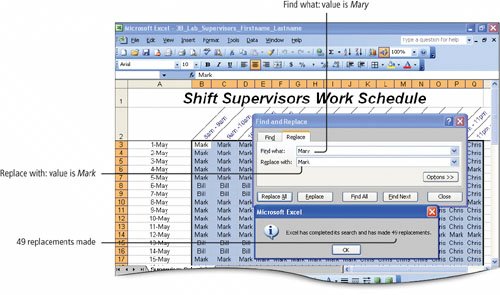
The Microsoft Excel dialog box displays and informs you that 49 replacements were made. |
|
4. |
Click OK. In the Find and Replace dialog box, click Close. Click any cell to deselect the range. Scroll down to view rows 35 through 42. Notice that Mary's hours are zero and Mark's hours now exceed the maximum of 248. Compare your screen with Figure 3.26. Figure 3.26. 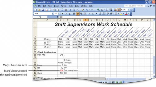
|
Objective 4 Use a Date Function |
Windows XP
- Chapter One. Getting Started with Windows XP
- Project 1A. Windows XP
- Objective 1. Get Started with Windows XP
- Objective 2. Resize, Move, and Scroll Windows
- Objective 3. Maximize, Restore, Minimize, and Close a Window
- Objective 4. Create a New Folder
- Objective 5. Copy, Move, Rename, and Delete Files
- Objective 6. Find Files and Folders
- Objective 7. Compress Files
- Summary
- Key Terms
- Concepts Assessments
Outlook 2003
- Chapter One. Getting Started with Outlook 2003
- Getting Started with Microsoft Office Outlook 2003
- Project 1A. Exploring Outlook 2003
- Objective 1. Start and Navigate Outlook
- Objective 2. Read and Respond to E-mail
- Objective 3. Store Contact and Task Information
- Objective 4. Work with the Calendar
- Objective 5. Delete Outlook Information and Close Outlook
- Summary
- Key Terms
- Concepts Assessments
- Skill Assessments
- Performance Assessments
- Mastery Assessments
- Problem Solving
- GO! with Help
Internet Explorer
- Chapter One. Getting Started with Internet Explorer
- Getting Started with Internet Explorer 6.0
- Project 1A. College and Career Information
- Objective 1. Start Internet Explorer and Identify Screen Elements
- Objective 2. Navigate the Internet
- Objective 3. Create and Manage Favorites
- Objective 4. Search the Internet
- Objective 5. Save and Print Web Pages
- Summary
- Key Terms
- Concepts Assessments
- Skill Assessments
- Performance Assessments
- Mastery Assessments
- Problem Solving
Computer Concepts
- Chapter One. Basic Computer Concepts
- Objective 1. Define Computer and Identify the Four Basic Computing Functions
- Objective 2. Identify the Different Types of Computers
- Objective 3. Describe Hardware Devices and Their Uses
- Objective 4. Identify Types of Software and Their Uses
- Objective 5. Describe Networks and Define Network Terms
- Objective 6. Identify Safe Computing Practices
- Summary
- In this Chapter You Learned How to
- Key Terms
- Concepts Assessments
Word 2003
Chapter One. Creating Documents with Microsoft Word 2003
- Chapter One. Creating Documents with Microsoft Word 2003
- Getting Started with Microsoft Office Word 2003
- Project 1A. Thank You Letter
- Objective 1. Create and Save a New Document
- Objective 2. Edit Text
- Objective 3. Select, Delete, and Format Text
- Objective 4. Create Footers and Print Documents
- Project 1B. Party Themes
- Objective 5. Navigate the Word Window
- Objective 6. Add a Graphic to a Document
- Objective 7. Use the Spelling and Grammar Checker
- Objective 8. Preview and Print Documents, Close a Document, and Close Word
- Objective 9. Use the Microsoft Help System
- Summary
- Key Terms
- Concepts Assessments
- Skill Assessments
- Performance Assessments
- Mastery Assessments
- Problem Solving
- You and GO!
- Business Running Case
- GO! with Help
Chapter Two. Formatting and Organizing Text
- Formatting and Organizing Text
- Project 2A. Alaska Trip
- Objective 1. Change Document and Paragraph Layout
- Objective 2. Change and Reorganize Text
- Objective 3. Create and Modify Lists
- Project 2B. Research Paper
- Objective 4. Insert and Format Headers and Footers
- Objective 5. Insert Frequently Used Text
- Objective 6. Insert and Format References
- Summary
- Key Terms
- Concepts Assessments
- Skill Assessments
- Performance Assessments
- Mastery Assessments
- Problem Solving
- You and GO!
- Business Running Case
- GO! with Help
Chapter Three. Using Graphics and Tables
- Using Graphics and Tables
- Project 3A. Job Opportunities
- Objective 1. Insert and Modify Clip Art and Pictures
- Objective 2. Use the Drawing Toolbar
- Project 3B. Park Changes
- Objective 3. Set Tab Stops
- Objective 4. Create a Table
- Objective 5. Format a Table
- Objective 6. Create a Table from Existing Text
- Summary
- Key Terms
- Concepts Assessments
- Skill Assessments
- Performance Assessments
- Mastery Assessments
- Problem Solving
- You and GO!
- Business Running Case
- GO! with Help
Chapter Four. Using Special Document Formats, Columns, and Mail Merge
- Using Special Document Formats, Columns, and Mail Merge
- Project 4A. Garden Newsletter
- Objective 1. Create a Decorative Title
- Objective 2. Create Multicolumn Documents
- Objective 3. Add Special Paragraph Formatting
- Objective 4. Use Special Character Formats
- Project 4B. Water Matters
- Objective 5. Insert Hyperlinks
- Objective 6. Preview and Save a Document as a Web Page
- Project 4C. Recreation Ideas
- Objective 7. Locate Supporting Information
- Objective 8. Find Objects with the Select Browse Object Button
- Project 4D. Mailing Labels
- Objective 9. Create Labels Using the Mail Merge Wizard
- Summary
- Key Terms
- Concepts Assessments
- Skill Assessments
- Performance Assessments
- Mastery Assessments
- Problem Solving
- You and GO!
- Business Running Case
- GO! with Help
Excel 2003
Chapter One. Creating a Worksheet and Charting Data
- Creating a Worksheet and Charting Data
- Project 1A. Tableware
- Objective 1. Start Excel and Navigate a Workbook
- Objective 2. Select Parts of a Worksheet
- Objective 3. Enter and Edit Data in a Worksheet
- Objective 4. Construct a Formula and Use the Sum Function
- Objective 5. Format Data and Cells
- Objective 6. Chart Data
- Objective 7. Annotate a Chart
- Objective 8. Prepare a Worksheet for Printing
- Objective 9. Use the Excel Help System
- Project 1B. Gas Usage
- Objective 10. Open and Save an Existing Workbook
- Objective 11. Navigate and Rename Worksheets
- Objective 12. Enter Dates and Clear Formats
- Objective 13. Use a Summary Sheet
- Objective 14. Format Worksheets in a Workbook
- Summary
- Key Terms
- Concepts Assessments
- Skill Assessments
- Performance Assessments
- Mastery Assessments
- Problem Solving
- You and GO!
- Business Running Case
- GO! with Help
Chapter Two. Designing Effective Worksheets
- Designing Effective Worksheets
- Project 2A. Staff Schedule
- Objective 1. Use AutoFill to Fill a Pattern of Column and Row Titles
- Objective 2. Copy Text Using the Fill Handle
- Objective 3. Use AutoFormat
- Objective 4. View, Scroll, and Print Large Worksheets
- Project 2B. Inventory Value
- Objective 5. Design a Worksheet
- Objective 6. Copy Formulas
- Objective 7. Format Percents, Move Formulas, and Wrap Text
- Objective 8. Make Comparisons Using a Pie Chart
- Objective 9. Print a Chart on a Separate Worksheet
- Project 2C. Population Growth
- Objective 10. Design a Worksheet for What-If Analysis
- Objective 11. Perform What-If Analysis
- Objective 12. Compare Data with a Line Chart
- Summary
- Key Terms
- Concepts Assessments
- Skill Assessments
- Performance Assessments
- Mastery Assessments
- Problem Solving
- You and GO!
- Business Running Case
- GO! with Help
Chapter Three. Using Functions and Data Tables
- Using Functions and Data Tables
- Project 3A. Geography Lecture
- Objective 1. Use SUM, AVERAGE, MIN, and MAX Functions
- Objective 2. Use a Chart to Make Comparisons
- Project 3B. Lab Supervisors
- Objective 3. Use COUNTIF and IF Functions, and Apply Conditional Formatting
- Objective 4. Use a Date Function
- Project 3C. Loan Payment
- Objective 5. Use Financial Functions
- Objective 6. Use Goal Seek
- Objective 7. Create a Data Table
- Summary
- Key Terms
- Concepts Assessments
- Skill Assessments
- Performance Assessments
- Mastery Assessments
- Problem Solving
- You and GO!
- Business Running Case
- GO! with Help
Access 2003
Chapter One. Getting Started with Access Databases and Tables
- Getting Started with Access Databases and Tables
- Project 1A. Academic Departments
- Objective 1. Rename a Database
- Objective 2. Start Access, Open an Existing Database, and View Database Objects
- Project 1B. Fundraising
- Objective 3. Create a New Database
- Objective 4. Create a New Table
- Objective 5. Add Records to a Table
- Objective 6. Modify the Table Design
- Objective 7. Create Table Relationships
- Objective 8. Find and Edit Records in a Table
- Objective 9. Print a Table
- Objective 10. Close and Save a Database
- Objective 11. Use the Access Help System
- Summary
- Key Terms
- Concepts Assessments
- Skill Assessments
- Performance Assessments
- Mastery Assessments
- Problem Solving Assessments
- Problem Solving
- You and GO!
- Business Running Case
- GO! with Help
Chapter Two. Sort, Filter, and Query a Database
- Sort, Filter, and Query a Database
- Project 2A. Club Fundraiser
- Objective 1. Sort Records
- Objective 2. Filter Records
- Objective 3. Create a Select Query
- Objective 4. Open and Edit an Existing Query
- Objective 5. Sort Data in a Query
- Objective 6. Specify Text Criteria in a Query
- Objective 7. Print a Query
- Objective 8. Specify Numeric Criteria in a Query
- Objective 9. Use Compound Criteria
- Objective 10. Create a Query Based on More Than One Table
- Objective 11. Use Wildcards in a Query
- Objective 12. Use Calculated Fields in a Query
- Objective 13. Group Data and Calculate Statistics in a Query
- Summary
- Key Terms
- Concepts Assessments
- Skill Assessments
- Performance Assessments
- Mastery Assessments
- Problem Solving
- You and GO!
- Business Running Case
- GO! with Access Help
Chapter Three. Forms and Reports
- Forms and Reports
- Project 3A. Fundraiser
- Objective 1. Create an AutoForm
- Objective 2. Use a Form to Add and Delete Records
- Objective 3. Create a Form Using the Form Wizard
- Objective 4. Modify a Form
- Objective 5. Create an AutoReport
- Objective 6. Create a Report Using the Report Wizard
- Objective 7. Modify the Design of a Report
- Objective 8. Print a Report and Keep Data Together
- Summary
- Key Terms
- Concepts Assessments
- Skill Assessments
- Performance Assessments
- Mastery Assessments
- Problem Solving
- You and GO!
- Business Running Case
- GO! with Help
Powerpoint 2003
Chapter One. Getting Started with PowerPoint 2003
- Getting Started with PowerPoint 2003
- Project 1A. Expansion
- Objective 1. Start and Exit PowerPoint
- Objective 2. Edit a Presentation Using the Outline/Slides Pane
- Objective 3. Format and Edit a Presentation Using the Slide Pane
- Objective 4. View and Edit a Presentation in Slide Sorter View
- Objective 5. View a Slide Show
- Objective 6. Create Headers and Footers
- Objective 7. Print a Presentation
- Objective 8. Use PowerPoint Help
- Summary
- Key Terms
- Concepts Assessments
- Skill Assessments
- Performance Assessments
- Mastery Assessments
- Problem Solving
- You and GO!
- Business Running Case
- GO! with Help
Chapter Two. Creating a Presentation
- Creating a Presentation
- Project 2A. Teenagers
- Objective 1. Create a Presentation
- Objective 2. Modify Slides
- Project 2B. History
- Objective 3. Create a Presentation Using a Design Template
- Objective 4. Import Text from Word
- Objective 5. Move and Copy Text
- Summary
- Key Terms
- Concepts Assessments
- Skill Assessments
- Performance Assessments
- Mastery Assessments
- Problem Solving
- You and GO!
- Business Running Case
- GO! with Help
Chapter Three. Formatting a Presentation
- Project 3A. Emergency
- Objective 1. Format Slide Text
- Objective 2. Modify Placeholders
- Objective 3. Modify Slide Master Elements
- Objective 4. Insert Clip Art
- Project 3B. Volunteers
- Objective 5. Apply Bullets and Numbering
- Objective 6. Customize a Color Scheme
- Objective 7. Modify the Slide Background
- Objective 8. Apply an Animation Scheme
- Summary
- Key Terms
- Concepts Assessments
- Skill Assessments
- Performance Assessments
- Mastery Assessments
- Problem Solving
- You and GO!
- Business Running Case
- GO! with Help
Integrated Projects
Chapter One. Using Access Data with Other Office Applications
- Chapter One. Using Access Data with Other Office Applications
- Introduction
- Project 1A. Meeting Slides
- Objective 1. Export Access Data to Excel
- Objective 2. Create a Formula in Excel
- Objective 3. Create a Chart in Excel
- Objective 4. Copy Access Data into a Word Document
- Objective 5. Copy Excel Data into a Word Document
- Objective 6. Insert an Excel Chart into a PowerPoint Presentation
Chapter Two. Using Tables in Word and Excel
- Chapter Two. Using Tables in Word and Excel
- Introduction
- Project 2A. Meeting Notes
- Objective 1. Plan a Table in Word
- Objective 2. Enter Data and Format a Table in Word
- Objective 3. Create a Table in Word from Excel Data
- Objective 4. Create Excel Worksheet Data from a Word Table
Chapter Three. Using Excel as a Data Source in a Mail Merge
- Chapter Three. Using Excel as a Data Source in a Mail Merge
- Introduction
- Project 3A. Mailing Labels
- Objective 1. Prepare a Mail Merge Document as Mailing Labels
- Objective 2. Choose an Excel Worksheet as a Data Source
- Objective 3. Produce and Save Merged Mailing Labels
- Objective 4. Open a Saved Main Document for Mail Merge
Chapter Four. Linking Data in Office Documents
- Chapter Four. Linking Data in Office Documents
- Introduction
- Project 4A. Weekly Sales
- Objective 1. Insert and Link in Word an Excel Object
- Objective 2. Format an Object in Word
- Objective 3. Open a Word Document That Includes a Linked Object, and Update Links
Chapter Five. Creating Presentation Content from Office Documents
EAN: 2147483647
Pages: 448
- Linking the IT Balanced Scorecard to the Business Objectives at a Major Canadian Financial Group
- Measuring and Managing E-Business Initiatives Through the Balanced Scorecard
- Governing Information Technology Through COBIT
- The Evolution of IT Governance at NB Power
- Governance Structures for IT in the Health Care Industry
