SMOOTHING IMPULSIVE NOISE
In practice we may be required to make precise measurements in the presence of high noise or interference. Without some sort of analog signal conditioning, or digital signal processing, it can be difficult to obtain stable and repeatable, measurements. This impulsive-noise smoothing trick, originally developed to detect microampere changes in milliampere signals, describes a smoothing algorithm that improves the stability of precision measurements in the presence of impulsive noise[70].
Practical noise reduction methods often involve multiple-sample averaging (block averaging) of a sequence of measured values, x(n), to compute a sequence of N-sample arithmetic means, M(q). As such, the block averaged sequence M(q) is defined by:

where the time index of the averaging process is q = 0, 1, 2, 3, etc. When N = 10 for example, for the first block of data (q = 0), time samples x(0) through x(9) are averaged to compute M(0). For the second block of data (q = 1), time samples x(10) through x(19) are averaged to compute M(1), and so on[71].
The following impulsive-noise smoothing algorithm processes a block of time-domain samples, obtained through periodic sampling, and the number of samples, N, may be varied according to individual needs and processing resources. The processing of a single block of N time samples proceeds as follows: collect N+2 samples of x(n), discard the maximum (most positive) and minimum (most negative) samples to obtain an N-sample block of data, and compute the arithmetic mean, M(q), of the N samples. Each sample in the block is then compared to the mean. The direction of each sample relative to the mean (greater than, or less than) is accumulated, as well as the cumulative magnitude of the deviation of the samples in one direction (which, by definition of the mean, equals that of the other direction). This data is used to compute a correction term that is added to the mean according to the following formula:
Equation 13-124

where A(q) is the corrected mean, M(q) is the arithmetic mean (average) from Eq. (13-123), Pos is the number of samples greater than M(q), and Neg is the number of samples less than M(q), and Dtotal is the sum of deviations from the mean (absolute values and one direction only). Dtotal, then, is the sum of the differences between the Pos samples and M(q).
For an example, consider a system acquiring 10 measured samples of 10, 10, 11, 9, 10, 10, 13, 10, 10, and 10. The mean is M = 10.3, the total number of samples positive is Pos = 2, and the total number of samples negative is Neg = 8 (so Pos–Neg = –6). The total deviation in either direction from the mean is 3.4 [using the eight samples less than the mean, (10.3–10) times 7 plus (10.3–9); or using the two samples greater than the mean, (13–10.3) plus (11–10.3)]. With Dtotal = 3.4, Eq. (13-124) yields an improved result of A = 10.096.
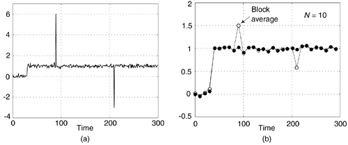
The smoothing algorithm's performance, relative to traditional block averaging, can be illustrated by example. Figure 13-71(a) shows a measured 300-sample x(n) signal sequence comprising a step signal of amplitude one contaminated with random noise (with a variance of 0.1) and two large impulsive-noise spike samples.
Figure 13-71. Noise smoothing for N = 10: (a) input x(n) signal; (b) block average output (white) and impulsive-noise smoothing algorithm output (solid).

A few meaningful issues regarding this noise smoothing process are:
- The block size (N) used in the smoothing algorithm can be any integer, but for real-time fixed binary-point implementations it's beneficial to set N equal to an integer power of two. In that case the compute-intensive division operations in Eq. (13-123) and Eq. (13-124) can be accomplished by binary arithmetic right shifts to reduce the computational workload.
- If there's a possibility that more than two large noise spikes are contained in a block of input samples, then we collect more than N+2 samples of x(n) and discard the appropriate number of maximum and minimum samples to eliminate the large impulsive noise samples.
- We could forego the Eq. (13-124) processing and merely perform Eq. (13-123) to compute the mean M(q). In that case, for a given N, the standard deviation of M(q) would be roughly 15–20% greater than A(q).
URL http://proquest.safaribooksonline.com/0131089897/ch13lev1sec25
 |
Amazon |  |
