A PRACTICAL SPECTRUM ANALYZER
Here's a clever trick for implementing a practical spectrum analyzer by modifying the time-domain data before applying a radix-2 FFT algorithm.
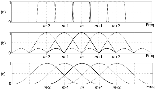
Let's say we need to build a spectrum analyzer to display, in some manner, the spectral magnitude of a time-domain sequence. We'd like our spectrum analyzer, a bank of bandpass filters, to have a frequency magnitude response something like that shown in Figure 13-55(a). For spectrum analysis, the radix-2 FFT algorithm comes to mind first, as it should. However, the frequency response of individual FFT bins is that shown in Figure 13-55(b), with their non-flat passbands, unpleasantly high sidelobes due to spectral leakage, and overlapped main lobes. We can reduce the leakage sidelobe levels by windowing the time-domain sequence, but that leads to the increased main lobe overlap shown in Figure 13-55(c) and degraded frequency resolution, and we still have considerable droop in the passband response.
Figure 13-55. Spectrum analyzer: (a) desired frequency response; (b) frequency response of standard FFT bins; (c) windowed-data FFT frequency response.

Here's how we can solve our problem. Consider an x(n) sequence of time samples of length M whose M-point DFT is

Next consider partitioning x(n) into P subsequences, each of length N. Thus PN = M. If we add, element for element, the P subsequences we'll obtain a new y(n) sequence of length N whose N-point DFT is
Equation 13-105

The good news is that
Equation 13-106

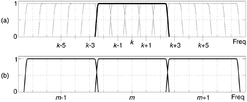
That is, the DFT magnitudes of sequence y(n) are equal to a subset of the longer DFT magnitudes of x(n). Y(m) is equal to a decimated-by-P version of X(k). The relationship between |Y(m)| and |X(Pm)| doesn't seem too important, but here's how we'll take advantage of that equality. We'll create an M-point window sequence whose single-bin frequency response, of an M-point FFT, is the bold curve in Figure 13-56(a). Instead of computing all M FFT outputs, we'll only compute every Pth output of the M-point FFT, implementing Eq. (13-105), giving us the decimated FFT bins shown in Figure 13-56(b). In that figure P = 5.
Figure 13-56. FFT spectrum analyzer frequency responses.

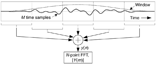
That decimation of the frequency-domain |X(k)| spectrum is accomplished in the time domain by a time-aliasing operation as shown in Figure 13-57 where again, for example, P = 5. We partition the M-sample windowed-x(n) time sequence into P = 5 subsequences, sum the subsequences element for element to obtain the time-aliased N-sample y(n) sequence. Next the |Y(m)| spectral magnitudes are computed using the radix-2 FFT. (With the input x(n) sequence being real-valued, with spectral symmetry, only N/2+1 the |Y(m)| magnitude values need be computed for display.)
Figure 13-57. FFT spectrum analyzer process.

This process, sweet in its simplicity, is called the weighted overlap-add structure[50,51], and is alternatively referred to as the window-presum FFT[52]. The most difficult part of building this analyzer is designing the M-point window sequence used to window the original x(n) sequence. We do that by specifying the window's frequency domain characteristics just as if it were a digital filter frequency response, and use our favorite filter design software to compute the filter's time-domain impulse response. That impulse response is the window sequence. With the signal sample rate being fs, the window's passband width will be just less than fs/N. This makes the filter's one-sided passband width roughly fs/2N.
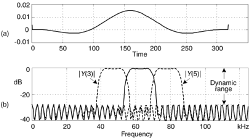
Figure 13-58 illustrates an example FFT analyzer with fs = 1 Mhz, N = 64, with P = 5 making M = 320. The FFT bin spacing is 15.63 kHz, so the window design was set for a passband width of 10 kHz (thus the filter's one-sided bandwidth was specified as 5 kHz in a Parks-McClellan design routine). Figure 13-58(a) is the 320-point window sequence, while Figure 13-58(b) shows FFT analyzer's response for the m = 3, 4, and 5 bins, with the |Y(4)| response being the solid curve.
Figure 13-58. FFT analyzer example: (a) window sequence; (b) analyzer response for 64-point FFT bins |Y(3)|, |Y(4)|, and |Y(5)|.

The width of the spectrum analyzer's passbands is primarily controlled by the window's passband width. The center frequencies of the analyzer's individual passbands is defined by fs/N. What this means is that the amount of overlap in the analyzer's passbands depends on both the window's passband width, fs, and N. The dynamic range of the analyzer can be increased by increasing P, which increases M and lengthens the x(n) sequence. As M is increased, the longer window sequence will yield analyzer passbands having a more rectangular shape, lower sidelobes, and reduced passband ripple.
Again, to implement this radix-2 FFT spectrum analyzer, the length of the time-domain sequence (M) must be an integer multiple (P) of an integer power of two (N).
URL http://proquest.safaribooksonline.com/0131089897/ch13lev1sec20
 |
Amazon |  |
