THE LAPLACE TRANSFORM
The Laplace transform is a mathematical method of solving linear differential equations that has proved very useful in the fields of engineering and physics. This transform technique, as it's used today, originated from the work of the brilliant English physicist Oliver Heaviside.[ ] The fundamental process of using the Laplace transform goes something like the following:
[
Step 1. A time-domain differential equation is written that describes the input/output relationship of a physical system (and we want to find the output function that satisfies that equation with a given input).
Step 2. The differential equation is Laplace transformed, converting it to an algebraic equation.
Step 3. Standard algebraic techniques are used to determine the desired output function's equation in the Laplace domain.
Step 4. The desired Laplace output equation is, then, inverse Laplace transformed to yield the desired time-domain output function's equation.
This procedure, at first, seems cumbersome because it forces us to go the long way around, instead of just solving a differential equation directly. The justification for using the Laplace transform is that although solving differential equations by classical methods is a very powerful analysis technique for all but the most simple systems, it can be tedious and (for some of us) error prone. The reduced complexity of using algebra outweighs the extra effort needed to perform the required forward and inverse Laplace transformations. This is especially true now that tables of forward and inverse Laplace transforms exist for most of the commonly encountered time functions. Well known properties of the Laplace transform also allow practitioners to decompose complicated time functions into combinations of simpler functions and, then, use the tables. (Tables of Laplace transforms allow us to translate quickly back and forth between a time function and its Laplace transform—analogous to, say, a German-English dictionary if we were studying the German language.[]) Let's briefly look at a few of the more important characteristics of the Laplace transform that will prove useful as we make our way toward the discrete z-transform used to design and analyze IIR digital filters.
[
The Laplace transform of a continuous time-domain function f(t), where f(t) is defined only for positive time (t > 0), is expressed mathematically as
F(s) is called "the Laplace transform of f(t)," and the variable s is the complex number
Equation 6-4

A more general expression for the Laplace transform, called the bilateral or two-sided transform, uses negative infinity (– ) as the lower limit of integration. However, for the systems that we'll be interested in, where system conditions for negative time (t < 0) are not needed in our analysis, the one-sided Eq. (6-3) applies. Those systems, often referred to as causal systems, may have initial conditions at t = 0 that must be taken into account (velocity of a mass, charge on a capacitor, temperature of a body, etc.) but we don't need to know what the system was doing prior to t = 0.
In Eq. (6-4), s is a real number and w is frequency in radians/ second. Because e–st is dimensionless, the exponent term s must have the dimension of 1/time, or frequency. That's why the Laplace variable s is often called a complex frequency.
To put Eq. (6-3) into words, we can say that it requires us to multiply, point for point, the function f(t) by the complex function e–st for a given value of s. (We'll soon see that using the function e–st here is not accidental; e–st is used because it's the general form for the solution of linear differential equations.) After the point-for-point multiplications, we find the area under the curve of the function f(t)e–st by summing all the products. That area, a complex number, represents the value of the Laplace transform for the particular value of s = s + jw chosen for the original multiplications. If we were to go through this process for all values of s, we'd have a full description of F(s) for every value of s.
I like to think of the Laplace transform as a continuous function, where the complex value of that function for a particular value of s is a correlation of f(t) and a damped complex e–st sinusoid whose frequency is w and whose damping factor is s. What do these complex sinusoids look like? Well, they are rotating phasors described by
Equation 6-5
From our knowledge of complex numbers, we know that e–jwt is a unity-magnitude phasor rotating clockwise around the origin of a complex plane at a frequency of w radians per second. The denominator of Eq. (6-5) is a real number whose value is one at time t = 0. As t increases, the denominator est gets larger (when s is positive), and the complex e–st phasor's magnitude gets smaller as the phasor rotates on the complex plane. The tip of that phasor traces out a curve spiraling in toward the origin of the complex plane. One way to visualize a complex sinusoid is to consider its real and imaginary parts individually. We do this by expressing the complex e–st sinusoid from Eq. (6-5) in rectangular form as
Equation 6-5'
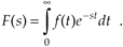
Figure 6-4 shows the real parts (cosine) of several complex sinusoids with different frequencies and different damping factors. In Figure 6-4(a), the complex sinusoid's frequency is the arbitrary w', and the damping factor is the arbitrary s'. So the real part of F(s), at s = s' + jw', is equal to the correlation of f(t) and the wave in Figure 6-4(a). For different values of s, we'll correlate f(t) with different complex sinusoids as shown in Figure 6-4. (As we'll see, this correlation is very much like the correlation of f(t) with various sine and cosine waves when we were calculating the discrete Fourier transform.) Again, the real part of F(s), for a particular value of s, is the correlation of f(t) with a cosine wave of frequency w and a damping factor of s, and the imaginary part of F(s) is the correlation of f(t) with a sinewave of frequency w and a damping factor of s.
Figure 6-4. Real part (cosine) of various e–st functions, where s = s + jw, to be correlated with f(t).
Now, if we associate each of the different values of the complex s variable with a point on a complex plane, rightfully called the s-plane, we could plot the real part of the F(s) correlation as a surface above (or below) that s-plane and generate a second plot of the imaginary part of the F(s) correlation as a surface above (or below) the s-plane. We can't plot the full complex F(s) surface on paper because that would require four dimensions. That's because s is complex, requiring two dimensions, and F(s) is itself complex and also requires two dimensions. What we can do, however, is graph the magnitude |F(s)| as a function of s because this graph requires only three dimensions. Let's do that as we demonstrate this notion of an |F(s)| surface by illustrating the Laplace transform in a tangible way.
Say, for example, that we have the linear system shown in Figure 6-5. Also, let's assume that we can relate the x(t) input and the y(t) output of the linear time invariant physical system in Figure 6-5 with the following messy homogeneous constant-coefficient differential equation
Equation 6-6
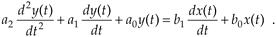
Figure 6-5. System described by Eq. (6-6). The system's input and output are the continuous time functions x(t) and y(t) respectively.
We'll use the Laplace transform toward our goal of figuring out how the system will behave when various types of input functions are applied, i.e., what the y(t) output will be for any given x(t) input.
Let's slow down here and see exactly what Figure 6-5 and Eq. (6-6) are telling us. First, if the system is time invariant, then the an and bn coefficients in Eq. (6-6) are constant. They may be positive or negative, zero, real or complex, but they do not change with time. If the system is electrical, the coefficients might be related to capacitance, inductance, and resistance. If the system is mechanical with masses and springs, the coefficients could be related to mass, coefficient of damping, and coefficient of resilience. Then, again, if the system is thermal with masses and insulators, the coefficients would be related to thermal capacity and thermal conductance. To keep this discussion general, though, we don't really care what the coefficients actually represent.
OK, Eq. (6-6) also indicates that, ignoring the coefficients for the moment, the sum of the y(t) output plus derivatives of that output is equal to the sum of the x(t) input plus the derivative of that input. Our problem is to determine exactly what input and output functions satisfy the elaborate relationship in Eq. (6-6). (For the stout hearted, classical methods of solving differential equations could be used here, but the Laplace transform makes the problem much simpler for our purposes.) Thanks to Laplace, the complex exponential time function of est is the one we'll use. It has the beautiful property that it can be differentiated any number of times without destroying its original form. That is
Equation 6-7

If we let x(t) and y(t) be functions of est, x(est) and y(est), and use the properties shown in Eq. (6-7), Eq. (6-6) becomes
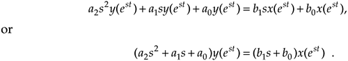
or
Equation 6-8

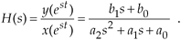
Although it's simpler than Eq. (6-6), we can further simplify the relationship in the last line in Eq. (6-8) by considering the ratio of y(est) over x(est) as the Laplace transfer function of our system in Figure 6-5. If we call that ratio of polynomials the transfer function H(s),
Equation 6-9
To indicate that the original x(t) and y(t) have the identical functional form of est, we can follow the standard Laplace notation of capital letters and show the transfer function as
Equation 6-10
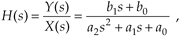
where the output Y(s) is given by
Equation 6-11
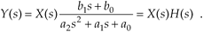
Equation (6-11) leads us to redraw the original system diagram in a form that highlights the definition of the transfer function H(s) as shown in Figure 6-6.
Figure 6-6. Linear system described by Eqs. (6-10) and (6-11). The system's input is the Laplace function X(s), its output is the Laplace function Y(s), and the system transfer function is H(s).
The cautious reader may be wondering, "Is it really valid to use this Laplace analysis technique when it's strictly based on the system's x(t) input being some function of est, or x(est)?" The answer is that the Laplace analysis technique, based on the complex exponential x(est), is valid because all practical x(t) input functions can be represented with complex exponentials. For example,
- a constant, c = ce0t ,
- sinusoids, sin(wt) = (ejwt – e–jwt)/2j or cos(wt) = (ejwt + e–jwt)/2 ,
- a monotonic exponential, eat, and
- an exponentially varying sinusoid, e–at cos(wt).
With that said, if we know a system's transfer function H(s), we can take the Laplace transform of any x(t) input to determine X(s), multiply that X(s) by H(s) to get Y(s), and then inverse Laplace transform Y(s) to yield the time-domain expression for the output y(t). In practical situations, however, we usually don't go through all those analytical steps because it's the system's transfer function H(s) in which we're most interested. Being able to express H(s) mathematically or graph the surface |H(s)| as a function of s will tell us the two most important properties we need to know about the system under analysis: Is the system stable, and if so, what is its frequency response?
"But wait a minute," you say. "Equations (6-10) and (6-11) indicate that we have to know the Y(s) output before we can determine H(s)!" Not really. All we really need to know is the time-domain differential equation like that in Eq. (6-6). Next we take the Laplace transform of that differential equation and rearrange the terms to get the H(s) ratio in the form of Eq. (6-10). With practice, systems designers can look at a diagram (block, circuit, mechanical, whatever) of their system and promptly write the Laplace expression for H(s). Let's use the concept of the Laplace transfer function H(s) to determine the stability and frequency response of simple continuous systems.
6.2.1 Poles and Zeros on the s-Plane and Stability
One of the most important characteristics of any system involves the concept of stability. We can think of a system as stable if, given any bounded input, the output will always be bounded. This sounds like an easy condition to achieve because most systems we encounter in our daily lives are indeed stable. Nevertheless, we have all experienced instability in a system containing feedback. Recall the annoying howl when a public address system's microphone is placed too close to the loudspeaker. A sensational example of an unstable system occurred in western Washington when the first Tacoma Narrows Bridge began oscillating on the afternoon of November 7th, 1940. Those oscillations, caused by 42 mph winds, grew in amplitude until the bridge destroyed itself. For IIR digital filters with their built-in feedback, instability would result in a filter output that's not at all representative of the filter input; that is, our filter output samples would not be a filtered version of the input; they'd be some strange oscillating or pseudorandom values. A situation we'd like to avoid if we can, right? Let's see how.
We can determine a continuous system's stability by examining several different examples of H(s) transfer functions associated with linear time-invariant systems. Assume that we have a system whose Laplace transfer function is of the form of Eq. (6-10), the coefficients are all real, and the coefficients b1 and a2 are equal to zero. We'll call that Laplace transfer function H1(s), where
Equation 6-12
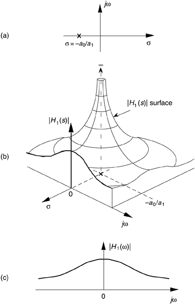
Notice that if s = –a0/a1, the denominator in Eq. (6-12) equals zero and H1(s) would have an infinite magnitude. This s = –a0/a1 point on the s-plane is called a pole, and that pole's location is shown by the "x" in Figure 6-7(a). Notice that the pole is located exactly on the negative portion of the real s axis. If the system described by H1 were at rest and we disturbed it with an impulse like x(t) input at time t = 0, its continuous time-domain y(t) output would be the damped exponential curve shown in Figure 6-7(b). We can see that H1(s) is stable because its y(t) output approaches zero as time passes. By the way, the distance of the pole from the s = 0 axis, a0/a1 for our H1(s), gives the decay rate of the y(t) impulse response. To illustrate why the term pole is appropriate, Figure 6-8(b) depicts the three-dimensional surface of |H1(s)| above the s-plane. Look at Figure 6-8(b) carefully and see how we've reoriented the s-plane axis. This new axis orientation allows us to see how the H1(s) system's frequency magnitude response can be determined from its three-dimensional s-plane surface. If we examine the |H1(s)| surface at s = 0, we get the bold curve in Figure 6-8(b). That bold curve, the intersection of the vertical s = 0 plane (the jw axis plane) and the |H1(s)| surface, gives us the frequency magnitude response |H1(w)| of the system—and that's one of the things we're after here. The bold |H1(w)| curve in Figure 6-8(b) is shown in a more conventional way in Figure 6-8(c). Figures 6-8(b) and 6-8(c) highlight the very important property that the Laplace transform is a more general case of the Fourier transform because if s = 0, then s = jw. In this case, the |H1(s)| curve for s = 0 above the s-plane becomes the |H1(w)| curve above the jw axis in Figure 6-8(c).
Figure 6-7. Descriptions of H1(s): (a) pole located at s = s + jw = –a0/a1 + j0 on the s-plane; (b) time-domain y(t) impulse response of the system.
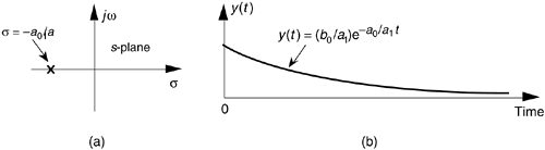
Figure 6-8. Further depictions of H1(s): (a) pole located at s = –a0/a1 on the s-plane; (b) |H1(s)| surface; (c) curve showing the intersection of the |H1(s)| surface and the vertical s = 0 plane. This is the conventional depiction of the |H1(w)| frequency magnitude response.
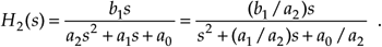
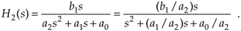
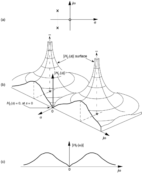
Another common system transfer function leads to an impulse response that oscillates. Let's think about an alternate system whose Laplace transfer function is of the form of Eq. (6-10), the coefficient b0 equals zero, and the coefficients lead to complex terms when the denominator polynomial is factored. We'll call this particular second-order transfer function H2(s), where
Equation 6-13
(By the way, when a transfer function has the Laplace variable s in both the numerator and denominator, the order of the overall function is defined by the largest exponential order of s in the denominator polynomial. So our H2(s) is a second-order transfer function.) To keep the following equations from becoming too messy, let's factor its denominator and rewrite Eq. (6-13) as
Equation 6-14
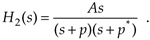
where A = b1/a2, p = preal + jpimag, and p* = preal – jpimag (complex conjugate of p). Notice that, if s is equal to –p or –p*, one of the polynomial roots in the denominator of Eq. (6-14) will equal zero, and H2(s) will have an infinite magnitude. Those two complex poles, shown in Figure 6-9(a), are located off the negative portion of the real s axis. If the H2 system were at rest and we disturbed it with an impulselike x(t) input at time t = 0, its continuous time-domain y(t) output would be the damped sinusoidal curve shown in Figure 6-9(b). We see that H2(s) is stable because its oscillating y(t) output, like a plucked guitar string, approaches zero as time increases. Again, the distance of the poles from the s = 0 axis (–preal) gives the decay rate of the sinusoidal y(t) impulse response. Likewise, the distance of the poles from the jw = 0 axis (±pimag) gives the frequency of the sinusoidal y(t) impulse response. Notice something new in Figure 6-9(a). When s = 0, the numerator of Eq. (6-14) is zero, making the transfer function H2(s) equal to zero. Any value of s where H2(s) = 0 is sometimes of interest and is usually plotted on the s-plane as the little circle, called a "zero," shown in Figure 6-9(a). At this point we're not very interested in knowing exactly what p and p* are in terms of the coefficients in the denominator of Eq. (6-13). However, an energetic reader could determine the values of p and p* in terms of a0, a1, and a2 by using the following well-known quadratic factorization formula: Given the second-order polynomial f(s) = as2 + bs + c, then f(s) can be factored as
Equation 6-15
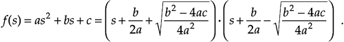
Figure 6-9. Descriptions of H2(s): (a) poles located at s = preal ± jpimag on the s-plane; (b) time domain y(t) impulse response of the system.
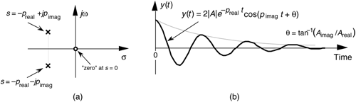
Figure 6-10(b) illustrates the |H2(s)| surface above the s-plane. Again, the bold |H2(w)| curve in Figure 6-10(b) is shown in the conventional way in Figure 6-10(c) to indicate the frequency magnitude response of the system described by Eq. (6-13). Although the three-dimensional surfaces in Figures 6-8(b) and 6-10(b) are informative, they're also unwieldy and unnecessary. We can determine a system's stability merely by looking at the locations of the poles on the two-dimensional s-plane.
Figure 6-10. Further depictions of H2(s): (a) poles and zero locations on the s–plane; (b) |H2(s)| surface; (c) |H2(w)| frequency magnitude response curve.
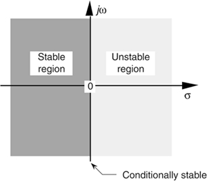
To further illustrate the concept of system stability, Figure 6-11 shows the s-plane pole locations of several example Laplace transfer functions and their corresponding time-domain impulse responses. We recognize Figures 6-11(a) and 6-11(b), from our previous discussion, as indicative of stable systems. When disturbed from their at-rest condition they respond and, at some later time, return to that initial condition. The single pole location at s = 0 in Figure 6-11(c) is indicative of the 1/s transfer function of a single element of a linear system. In an electrical system, this 1/s transfer function could be a capacitor that was charged with an impulse of current, and there's no discharge path in the circuit. For a mechanical system, Figure 6-11(c) would describe a kind of spring that's compressed with an impulse of force and, for some reason, remains under compression. Notice, in Figure 6-11(d), that, if an H(s) transfer function has conjugate poles located exactly on the jw axis (s = 0), the system will go into oscillation when disturbed from its initial condition. This situation, called conditional stability, happens to describe the intentional transfer function of electronic oscillators. Instability is indicated in Figures 6-11(e) and 6-11(f). Here, the poles lie to the right of the jw axis. When disturbed from their initial at-rest condition by an impulse input, their outputs grow without bound.[] See how the value of s, the real part of s, for the pole locations is the key here? When s < 0, the system is well behaved and stable; when s = 0, the system is conditionally stable; and when s > 0 the system is unstable. So we can say that, when s is located on the right half of the s-plane, the system is unstable. We show this characteristic of linear continuous systems in Figure 6-12. Keep in mind that real-world systems often have more than two poles, and a system is only as stable as its least stable pole. For a system to be stable, all of its transfer-function poles must lie on the left half of the s-plane.
[
Figure 6-11. Various H(s) pole locations and their time-domain impulse responses: (a) single pole at s < 0; (b) conjugate poles at s < 0; (c) single pole located at s = 0; (d) conjugate poles located at s = 0; (e) single pole at s > 0; (f) conjugate poles at s > 0.
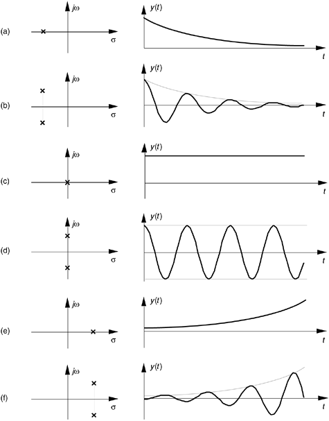
Figure 6-12. The Laplace s–plane showing the regions of stability and instability for pole locations for linear continuous systems.
To consolidate what we've learned so far: H(s) is determined by writing a linear system's time-domain differential equation and taking the Laplace transform of that equation to obtain a Laplace expression in terms of X(s), Y(s), s, and the system's coefficients. Next we rearrange the Laplace expression terms to get the H(s) ratio in the form of Eq. (6-10). (The really slick part is that we do not have to know what the time-domain x(t) input is to analyze a linear system!) We can get the expression for the continuous frequency response of a system just by substituting jw for s in the H(s) equation. To determine system stability, the denominator polynomial of H(s) is factored to find each of its roots. Each root is set equal to zero and solved for s to find the location of the system poles on the s-plane. Any pole located to the right of the jw axis on the s-plane will indicate an unstable system.
OK, returning to our original goal of understanding the z-transform, the process of analyzing IIR filter systems requires us to replace the Laplace transform with the z-transform and to replace the s-plane with a z-plane. Let's introduce the z-transform, determine what this new z-plane is, discuss the stability of IIR filters, and design and analyze a few simple IIR filters.
URL http://proquest.safaribooksonline.com/0131089897/ch06lev1sec2
| Amazon | ||
