BILINEAR TRANSFORM IIR FILTER DESIGN METHOD
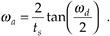
There's a popular analytical IIR filter design technique known as the bilinear transform method. Like the impulse invariance method, this design technique approximates a prototype analog filter defined by the continuous Laplace transfer function Hc(s) with a discrete filter whose transfer function is H(z). However, the bilinear transform method has great utility because
- it allows us simply to substitute a function of z for s in Hc(s) to get H(z), thankfully, eliminating the need for Laplace and z-transformations as well as any necessity for partial fraction expansion algebra;
- it maps the entire s-plane to the z-plane, enabling us to completely avoid the frequency-domain aliasing problems we had with the impulse invariance design method; and
- it induces a nonlinear distortion of H(z)'s frequency axis, relative to the original prototype analog filter's frequency axis, that sharpens the final roll-off of digital low-pass filters.
Don't worry. We'll explain each one of these characteristics and see exactly what they mean to us as we go about designing an IIR filter.
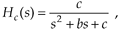
If the transfer function of a prototype analog filter is Hc(s), then we can obtain the discrete IIR filter z-domain transfer function H(z) by substituting the following for s in Hc(s)

where, again, ts is the discrete filter's sampling period (1/fs). Just as in the impulse invariance design method, when using the bilinear transform method, we're interested in where the analog filter's poles end up on the z-plane after the transformation. This s-plane to z-plane mapping behavior is exactly what makes the bilinear transform such an attractive design technique.[ ]
]
[
Let's investigate the major characteristics of the bilinear transform's s-plane to z-plane mapping. First we'll show that any pole on the left side of the s-plane will map to the inside of the unit circle in the z-plane. It's easy to show this by solving Eq. (6-88) for z in terms of s. Multiplying Eq. (6-88) by (ts/2)(1 + z–1) and collecting like terms of z leads us to
Equation 6-89

If we designate the real and imaginary parts of s as
Equation 6-90

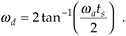
where the subscript in the radian frequency wa signifies analog, Eq. (6-89) becomes
Equation 6-91
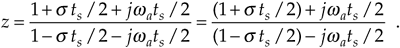
We see in Eq. (6-91) that z is complex, comprising the ratio of two complex expressions. As such, if we denote z as a magnitude at an angle in the form of z = |z| qz, we know that the magnitude of z is given by
Equation 6-92
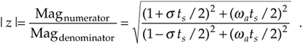
OK, if s is negative (s < 0) the numerator of the ratio on the right side of Eq. (6-92) will be less than the denominator, and |z| will be less than 1. On the other hand, if s is positive (s > 0), the numerator will be larger than the denominator, and |z| will be greater than 1. This confirms that, when using the bilinear transform defined by Eq. (6-88), any pole located on the left side of the s-plane (s < 0) will map to a z-plane location inside the unit circle. This characteristic ensures that any stable s-plane pole of a prototype analog filter will map to a stable z-plane pole for our discrete IIR filter. Likewise, any analog filter pole located on the right side of the s-plane (s > 0) will map to a z-plane location outside the unit circle when using the bilinear transform. This reinforces our notion that, to avoid filter instability, during IIR filter design, we should avoid allowing any z-plane poles to lie outside the unit circle.
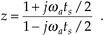
Next, let's show that the jwa axis of the s-plane maps to the perimeter of the unit circle in the z-plane. We can do this by setting s = 0 in Eq. (6-91) to get
Equation 6-93
Here, again, we see in Eq. (6-93) that z is a complex number comprising the ratio of two complex numbers, and we know the magnitude of this z is given by
Equation 6-94
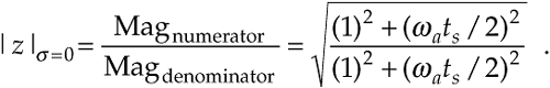
The magnitude of z in Eq. (6-94) is always 1. So, as we stated, when using the bilinear transform, the jwa axis of the s-plane maps to the perimeter of the unit circle in the z-plane. However, this frequency mapping from the s-plane to the unit circle in the z-plane is not linear. It's important to know why this frequency nonlinearity, or warping, occurs and to understand its effects. So we shall, by showing the relationship between the s-plane frequency and the z-plane frequency that we'll designate as wd.
If we define z on the unit circle in polar form as  as we did for Figure 6-13, where r is 1 and wd is the angle, we can substitute
  in Eq. (6-88) as
Equation 6-95
If we show s in its rectangular form and partition the ratio in brackets into half-angle expressions,
Equation 6-96

Using Euler's relationships of sin(ø) = (ejø – e–jø)/2j and cos(ø) = (ejø + e–jø)/2, we can convert the right side of Eq. (6-96) to rectangular form as
Equation 6-97
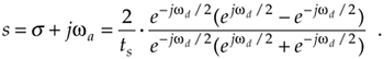
If we now equate the real and imaginary parts of Eq. (6-97), we see that s = 0, and
Equation 6-98
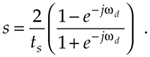
Let's rearrange Eq. (6-98) to give us the useful expression for the z-domain frequency wd, in terms of the s-domain frequency wa, of
Equation 6-99
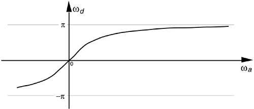
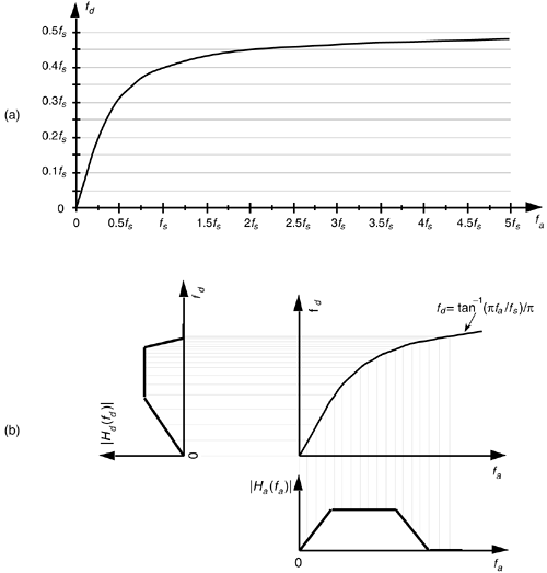
The important relationship in Eq. (6-99), which accounts for the so-called frequency warping due to the bilinear transform, is illustrated in Figure 6-30. Notice that, because tan–1(wats/2) approaches p/2 as wa gets large, wd must, then, approach twice that value, or p. This means that no matter how large wa gets, the z-plane wd will never be greater than p.
Figure 6-30. Nonlinear relationship between the z-domain frequency wd and the s-domain frequency wa.
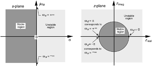
Remember how we considered Figure 6-14 and stated that only the –pfs to +pfs radians/s frequency range for wa can be accounted for on the z-plane? Well, our new mapping from the bilinear transform maps the entire s-plane to the z-plane, not just the primary strip of the s-plane shown in Figure 6-14. Now, just as a walk along the jwa frequency axis on the s-plane takes us to infinity in either direction, a trip halfway around the unit circle in a counterclockwise direction takes us from wa = 0 to wa = + radians/s. As such, the bilinear transform maps the s-plane's entire jwa axis onto the unit circle in the z-plane. We illustrate these bilinear transform mapping properties in Figure 6-31.
Figure 6-31. Bilinear transform mapping of the s-plane to the z-plane.
To show the practical implications of this frequency warping, let's relate the s-plane and z-plane frequencies to the more practical measure of the fs sampling frequency. We do this by remembering the fundamental relationship between radians/s and Hz of w = 2pf and solving for f to get
Equation 6-100

Applying Eq. (6-100) to Eq. (6-99),
Equation 6-101
Substituting 1/fs for ts, we solve Eq. (6-101) for fd to get
Equation 6-102
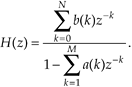
Equation (6-102), the relationship between the s-plane frequency fa in Hz and the z-plane frequency fd in Hz, is plotted in Figure 6-32(a) as a function of the IIR filter's sampling rate fs.
Figure 6-32. Nonlinear relationship between the fd and fc frequencies: (a) frequency warping curve scaled in terms of the IIR filter's fs sampling rate; (b) s-domain frequency response Hc(fc) transformation to a z-domain frequency response Hd(fd).
The distortion of the fa frequency scale, as it translates to the fd frequency scale, is illustrated in Figure 6-32(b), where an s-plane bandpass frequency magnitude response |Ha(fa)| is subjected to frequency compression as it is transformed to |Hd(fd)|. Notice how the low-frequency portion of the IIR filter's |Hd(fd)| response is reasonably linear, but the higher frequency portion has been squeezed in toward zero Hz. That's frequency warping. This figure shows why no IIR filter aliasing can occur with the bilinear transform design method. No matter what the shape or bandwidth of the |Ha(fa)| prototype analog filter, none of its spectral content can extend beyond half the sampling rate of fs/2 in |Hd(fd)—and that's what makes the bilinear transform design method as popular as it is.
The steps necessary to perform an IIR filter design using the bilinear transform method are as follows:
Step 1. Obtain the Laplace transfer function Hc(s) for the prototype analog filter in the form of Eq. (6-43).
Step 2. Determine the digital filter's equivalent sampling frequency fs and establish the sample period ts = 1/fs.
Step 3. In the Laplace Hc(s) transfer function, substitute the expression
Equation 6-103

for the variable s to get the IIR filter's H(z) transfer function.
Step 4. Multiply the numerator and denominator of H(z) by the appropriate power of (1 + z–1) and grind through the algebra to collect terms of like powers of z in the form
Equation 6-104
Step 5. Just as in the impulse invariance design methods, by inspection, we can express the IIR filter's time-domain equation in the general form of
Equation 6-105
Although the expression in Eq. (6-105) only applies to the filter structure in Figure 6-18, to complete our design, we can apply the a(k) and b(k) coefficients to the improved IIR structure shown in Figure 6-22.
To show just how straightforward the bilinear transform design method is, let's use it to solve the IIR filter design problem first presented for the impulse invariance design method.
6.5.1 Bilinear Transform Design Example
Again, our goal is to design an IIR filter that approximates the second-order Chebyshev prototype analog low-pass filter, shown in Figure 6-26, whose passband ripple is 1 dB. The fs sampling rate is 100 Hz (ts = 0.01), and the filter's 1 dB cutoff frequency is 20 Hz. As before, given the original prototype filter's Laplace transfer function as
Equation 6-106
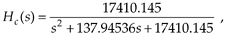
and the value of ts = 0.01 for the sample period, we're ready to proceed with Step 3. For convenience, let's replace the constants in Eq. (6-106) with variables in the form of
Equation 6-107
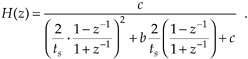
where b = 137.94536 and c = 17410.145. Performing the substitution of Eq. (6-103) in Eq. (6-107),
Equation 6-108
To simplify our algebra a little, let's substitute the variable a for the fraction 2/ts to give
Equation 6-109
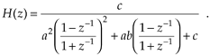
Proceeding with Step 4, we multiply Eq. (109)'s numerator and denominator by (1 + z–1)2 to yield
Equation 6-110
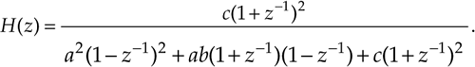
Multiplying through by the factors in the denominator of Eq. (6-110), and collecting like powers of z,
Equation 6-111
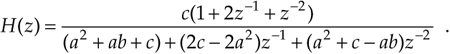
We're almost there. To get Eq. (6-111) into the form of Eq. (6-104) with a constant term of one in the denominator, we divide Eq. (6-111)'s numerator and denominator by (a2 + ab + c), giving us
Equation 6-112
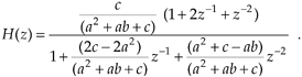
We now have H(z) in a form with all the like powers of z combined into single terms, and Eq. (6-112) looks something like the desired form of Eq. (6-104). If we plug the values a = 2/ts = 200, b = 137.94536, and c = 17410.145 into Eq. (6-112) we get the following IIR filter transfer function:
Equation 6-113
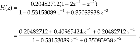
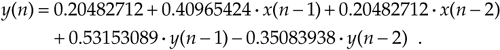
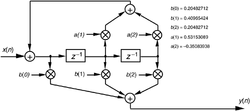
and there we are. Now, by inspection of Eq. (6-113), we get the time-domain expression for our IIR filter as
Equation 6-114
The frequency magnitude response of our bilinear transform IIR design example is shown as the dark curve in Figure 6-33(a), where, for comparison, we've shown the result of that impulse invariance design example as the shaded curve. Notice how the bilinear transform designed filter's magnitude response approaches zero at the folding frequency of fs/2 = 50 Hz. This is as it should be—that's the whole purpose of the bilinear transform design method. Figure 6-33(b) illustrates the nonlinear phase response of the bilinear transform designed IIR filter.
Figure 6-33. Comparison of the bilinear transform and impulse invariance design IIR filters: (a) frequency magnitude responses; (b) phase of the bilinear transform IIR filter.
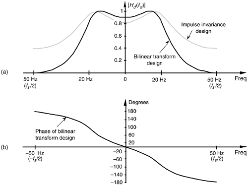
We might be tempted to think that not only is the bilinear transform design method easier to perform than the impulse invariance design method, but that it gives us a much sharper roll-off for our low-pass filter. Well, the frequency warping of the bilinear transform method does compress (sharpen) the roll-off portion of a low-pass filter, as we saw in Figure 6-32, but an additional reason for the improved response is the price we pay in terms of the additional complexity of the implementation of our IIR filter. We see this by examining the implementation of our IIR filter as shown in Figure 6-34. Notice that our new filter requires five multiplications per filter output sample where the impulse invariance design filter in Figure 6-28(a) required only three multiplications per filter output sample. The additional multiplications are, of course, required by the additional feed forward z terms in the numerator of Eq. (6-113). These added b(k) coefficient terms in the H(z) transfer function correspond to zeros in the z-plane created by the bilinear transform that did not occur in the impulse invariance design method.
Figure 6-34. Implementation of the bilinear transform design example filter.
Because our example prototype analog low-pass filter had a cutoff frequency that was fs/5, we don't see a great deal of frequency warping in the bilinear transform curve in Figure 6-33. (In fact, Kaiser has shown that, when fs is large, the impulse invariance and bilinear transform design methods result in essentially identical H(z) transfer functions[19].) Had our cutoff frequency been a larger percentage of fs, bilinear transform warping would have been more serious, and our resultant |Hd(fd)| cutoff frequency would have been below the desired value. What the pros do to avoid this is to prewarp the prototype analog filter's cutoff frequency requirement before the analog Hc(s) transfer function is derived in Step 1.
In that way, they compensate for the bilinear transform's frequency warping before it happens. We can use Eq. (6-98) to determine the prewarped prototype analog filter low-pass cutoff frequency that we want mapped to the desired IIR low-pass cutoff frequency. We plug the desired IIR cutoff frequency wd in Eq. (6-98) to calculate the prototype analog wa cutoff frequency used to derive the prototype analog filter's Hc(s) transfer function.
Although we explained how the bilinear transform design method avoided the impulse invariance method's inherent frequency response aliasing, it's important to remember that we still have to avoid filter input data aliasing. No matter what kind of digital filter or filter design method is used, the original input signal data must always be obtained using a sampling scheme that avoids the aliasing described in Chapter 2. If the original input data contains errors due to sample rate aliasing, no filter can remove those errors.
Our introductions to the impulse invariance and bilinear transform design techniques have, by necessity, presented only the essentials of those two design methods. Although rigorous mathematical treatment of the impulse invariance and bilinear transform design methods is inappropriate for an introductory text such as this, more detailed coverage is available to the interested reader[13–16]. References [13] and [15], by the way, have excellent material on the various prototype analog filter types used as a basis for the analytical IIR filter design methods. Although our examples of IIR filter design using the impulse invariance and bilinear transform techniques approximated analog low-pass filters, it's important to remember that these techniques apply equally well to designing bandpass and highpass IIR filters. To design a highpass IIR filter, for example, we'd merely start our design with a Laplace transfer function for the prototype analog highpass filter. Our IIR digital filter design would then proceed to approximate that prototype highpass filter.
As we have seen, the impulse invariance and bilinear transform design techniques are both powerful and a bit difficult to perform. The mathematics is intricate and the evaluation of the design equations is arduous for all but the simplest filters. As such, we'll introduce a third class of IIR filter design methods based on software routines that take advantage of iterative optimization computing techniques. In this case, the designer defines the desired filter frequency response, and the algorithm begins generating successive approximations until the IIR filter coefficients converge (hopefully) to an optimized design.
URL http://proquest.safaribooksonline.com/0131089897/ch06lev1sec5
| Amazon | ||
