COMPUTING FFT TWIDDLE FACTORS
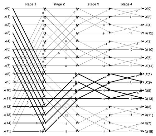
Typical applications using an N-point radix-2 FFT accept N input time samples, x(n), and compute N frequency-domain samples X(m). However, there are non-standard FFT applications (for example, specialized harmonic analysis, or perhaps using an FFT to implement a bank of filters) where only a subset of the X(m) results are required. Consider Figure 13-39 showing a 16-point radix-2 decimation in time FFT, and assume we only need to compute the X(1), X(5), X(9) and X(13) output samples. In this case, rather than compute the entire FFT we only need perform the computations indicated by the heavy lines. Reduced-computation FFTs are often called pruned FFTs[39–42]. (As we did in Chapter 4, for simplicity the butterflies in Figure 13-39 only show the twiddle phase angle factors and not the entire twiddle phase angles.) To implement pruned FFTs, we need to know the twiddle phase angles associated with each necessary butterfly computation as shown in Figure 13-40(a). Here we give an interesting algorithm for computing the 2pA1/N and 2pA2/N twiddle phase angles for an arbitrary-size FFT[43].
Figure 13-39. 16-point radix-2 FFT signal flow diagram.
The algorithm draws upon the following characteristics of a radix-2 decimation-in-time FFT:
- A general FFT butterfly is that shown in Figure 13-40(a).
Figure 13-40. Two forms of a radix-2 butterfly.
- The A1 and A2 angle factors are the integer values shown in Figure 13-39.
- An N-point radix-2 FFT has M stages (shown at the top of Figure 13-39) where M = log2(N).
- Each stage comprises N/2 butterflies.
The A1 phase angle factor of an arbitrary butterfly is
where S is the index of the M stages over the range 1  S M. Similarly, B serves as the index for the N/2 butterflies in each stage, where 1 B N/2. B = 1 means the top butterfly within a stage. The
  q
q operation is a function that returns the smallest integer q. Brev[z] represents the three-step operation of: convert decimal integer z to a binary number represented by M–1 binary bits, perform bit reversal on the binary number as discussed in Section 4.5, and convert the bit reversed number back to a decimal integer yielding angle factor A1. Angle factor A2, in Figure 13-40(a), is then computed using
Equation 13-76'

The algorithm can also be used to compute the single twiddle angle factor of the optimized butterfly shown in Figure 13-40(b). Below is a code listing, in MATLAB, implementing our twiddle angle factor computational algorithm.
clear
N = 16; %FFT size
M = log2(N); %Number of stages
Sstart = 1; %First stage to compute
Sstop = M; %Last stage to compute
Bstart = 1; %First butterfly to compute
Bstop = N/2; %Last butterfly to compute
Pointer = 0; %Init Results pointer
for S = Sstart:Sstop
 for B = Bstart:Bstop
 Z = floor((2^S*(B–1))/N); %Compute integer z
 % Compute bit reversal of Z
 Zbr = 0;
 for I = M–2:–1:0
 if Z>=2^I
 Zbr = Zbr + 2^(M–I–2);
 Z = Z –2^I;
 end
 end %End bit reversal
 A1 = Zbr; %Angle factor A1
 A2 = Zbr + N/2; %Angle factor A2
 Pointer = Pointer +1;
 Results(Pointer,:) = [S,B,A1,A2];
 end
end
Results, disp(' Stage B–fly, A1, A2'), disp(' ')
The variables in the code with start and stop in their names allow computation of a subset of the of all the twiddle angle factors in an N-point FFT. For example, to compute the twiddle angle factors for the fifth and sixth butterflies in the third stage of a 32-point FFT, we can assign N = 32, Sstart = 3, Sstop = 3, Bstart = 5, and Bstop = 6, and run the code.
URL http://proquest.safaribooksonline.com/0131089897/ch13lev1sec16
| Amazon | ||
