EFFICIENTLY PERFORMING THE FFT OF REAL SEQUENCES | Chapter Thirteen. Digital Signal Processing Tricks

Upon recognizing its linearity property and understanding the odd and even symmetries of the transform's output, the early investigators of the fast Fourier transform (FFT) realized that two separate, real N-point input data sequences could be transformed using a single N-point complex FFT. They also developed a technique using a single N-point complex FFT to transform a 2N-point real input sequence. Let's see how these two techniques work.

13.5.1 Performing Two N-Point Real FFTs

The standard FFT algorithms were developed to accept complex inputs; that is, the FFT's normal input x(n) sequence is assumed to comprise real and imaginary parts, such as

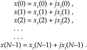
In typical signal processing schemes, FFT input data sequences are usually real. The most common example of this is the FFT input samples coming from an A/D converter that provides real integer values of some continuous (analog) signal. In this case the FFT's imaginary xi(n)'s inputs are all zero. So initial FFT computations performed on the xi(n) inputs represent wasted operations. Early FFT pioneers recognized this inefficiency, studied the problem, and developed a technique where two independent N-point, real input data sequences could be transformed by a single N-point complex FFT. We call this scheme the Two N-Point Real FFTs algorithm. The derivation of this technique is straightforward and described in the literature[17–19]. If two N-point, real input sequences are a(n) and b(n), they'll have discrete Fourier transforms represented by Xa(m) and Xb(m). If we treat the a(n) sequence as the real part of an FFT input and the b(n) sequence as the imaginary part of the FFT input, then

Equation 13-18

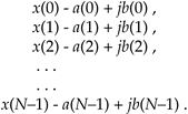
Applying the x(n) values from Eq. (13-18) to the standard DFT,

Equation 13-19

we'll get an DFT output X(m) where m goes from 0 to N–1. (We're assuming, of course, that the DFT is implemented by way of an FFT algorithm.) Using the superscript * symbol to represent the complex conjugate, we can extract the two desired FFT outputs Xa(m) and Xb(m) from X(m) by using the following:

Equation 13-20

and

Equation 13-21

Let's break Eqs. (13-20) and (13-21) into their real and imaginary parts to get expressions for Xa(m) and Xb(m) that are easier to understand and implement. Using the notation showing X(m)'s real and imaginary parts, where X(m) = Xr(m) + jXi(m), we can rewrite Eq. (13-20) as

Equation 13-22

where m = 1, 2, 3, . . ., N–1. What about the first Xa(m), when m = 0? Well, this is where we run into a bind if we actually try to implement Eq. (13-20) directly. Letting m = 0 in Eq. (13-40), we quickly realize that the first term in the numerator, X*(N–0) = X*(N), isn't available because the X(N) sample does not exist in the output of an N-point FFT! We resolve this problem by remembering that X(m) is periodic with a period N, so X(N) = X(0).[] When m = 0, Eq. (13-20) becomes

[] This fact is illustrated in Section 3.8 during the discussion of spectral leakage in DFTs.

Equation 13-23

Next, simplifying Eq. (13-21),

Equation 13-24

where, again, m = 1, 2, 3, . . ., N–1. By the same argument used for Eq. (13-23), when m = 0, Xb(0) in Eq. (13-24) becomes

Equation 13-25

This discussion brings up a good point for beginners to keep in mind. In the literature Eqs. (13-20) and (13-21) are often presented without any discussion of the m = 0 problem. So, whenever you're grinding through an algebraic derivation or have some equations tossed out at you, be a little skeptical. Try the equations out on an example—see if they're true. (After all, both authors and book typesetters are human and sometimes make mistakes. We had an old saying in Ohio for this situation: "Trust everybody, but cut the cards.") Following this advice, let's prove that this Two N-Point Real FFTs algorithm really does work by applying the 8-point data sequences from Chapter 3's DFT Examples to Eqs. (13-22) through (13-25). Taking the 8-point input data sequence from Section 3.1's DFT Example 1 and denoting it a(n),

Equation 13-26

Taking the 8-point input data sequence from Section 3.6's DFT Example 2 and calling it b(n),

Equation 13-27

Combining the sequences in Eqs. (13-26) and (13-27) into a single complex sequence x(n),

Equation 13-28

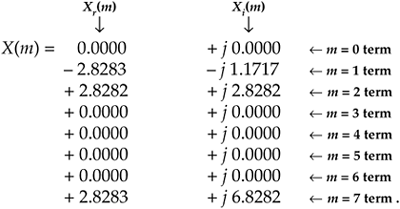
Now, taking the 8-point FFT of the complex sequence in Eq. (13-28) we get

Equation 13-29

So from Eq. (13-23),

To get the rest of Xa(m), we have to plug the FFT output's X(m) and X(N–m) values into Eq. (13-22).[] Doing so,

[] Remember, when the FFT's input is complex, the FFT outputs may not be conjugate symmetric; that is, we can't assume that F(m) is equal to F*(N–m) when the FFT input sequence's real and imaginary parts are both nonzero.

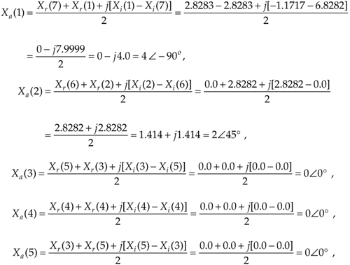
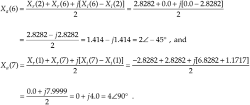
So Eq. (13-22) really does extract Xa(m) from the X(m) sequence in Eq. (13-29). We can see that we need not solve Eq. (13-22) when m is greater than 4 (or N/2) because Xa(m) will always be conjugate symmetric. Because Xa(7) = Xa(1), Xa(6) = Xa(2), etc., only the first N/2 elements in Xa(m) are independent and need be calculated.

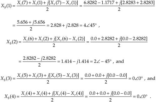
OK, let's keep going and use Eqs. (13-24) and (13-25) to extract Xb(m) from the FFT output. From Eq. (13-25),

Plugging the FFT's output values into Eq. (13-24) to get the next four Xb(m)s, we have

The question arises "With the additional processing required by Eqs. (13-22) and (13-24) after the initial FFT, how much computational saving (or loss) is to be had by this Two N-Point Real FFTs algorithm?" We can estimate the efficiency of this algorithm by considering the number of arithmetic operations required relative to two separate N-point radix-2 FFTs. First, we estimate the number of arithmetic operations in two separate N-point complex FFTs.

From Section 4.2, we know that a standard radix-2 N-point complex FFT comprises (N/2) log2N butterfly operations. If we use the optimized butterfly structure, each butterfly requires one complex multiplication and two complex additions. Now, one complex multiplication requires two real additions and four real multiplications, and one complex addition requires two real additions.[] So a single FFT butterfly operation comprises four real multiplications and six real additions. This means that a single N-point complex FFT requires (4N/2)·log2N real multiplications, and (6N/2)·log2N real additions. Finally, we can say that two separate N-point complex radix-2 FFTs require

[] The complex addition (a+jb) + (c+jd) = (a+c) + j(b+d) requires two real additions. A complex multiplication (a+jb) • (c+jd) = ac–bd + j(ad+bc) requires two real additions and four real multiplications.

Equation 13-30

Equation 13-30'

Next, we need to determine the computational workload of the Two N-Point Real FFTs algorithm. If we add up the number of real multiplications and real additions required by the algorithm's N-point complex FFT, plus those required by Eq. (13-22) to get Xa(m), and those required by Eq. (13-24) to get Xb(m), the Two N-Point Real FFTs algorithm requires

Equation 13-31

Equation 13-31'

Equations (13-31) and (13-31') assume that we're calculating only the first N/2 independent elements of Xa(m) and Xb(m). The single N term in Eq. (13-31) accounts for the N/2 divide by 2 operations in Eq. (13-22) and the N/2 divide by 2 operations in Eq. (13-24).

OK, now we can find out how efficient the Two N-Point Real FFTs algorithm is compared to two separate complex N-point radix-2 FFTs. This comparison, however, depends on the hardware used for the calculations. If our arithmetic hardware takes many more clock cycles to perform a multiplication than an addition, then the difference between multiplications in Eqs. (13-30) and (13-31) is the most important comparison. In this case, the percentage gain in computational saving of the Two N-Point Real FFTs algorithm relative to two separate N-point complex FFTs is the difference in their necessary multiplications over the number of multiplications needed for two separate N-point complex FFTs, or

Equation 13-32

The computational (multiplications only) saving from Eq. (13-32) is plotted as the top curve of Figure 13-11. In terms of multiplications, for N32, the Two N-Point Real FFTs algorithm saves us over 45 percent in computational workload compared to two separate N-point complex FFTs.

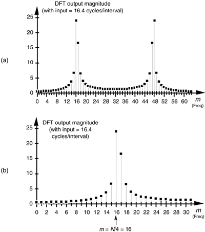
Figure 13-11. Computational saving of the Two N-Point Real FFTs algorithm over that of two separate N-point complex FFTs. The top curve indicates the saving when only multiplications are considered. The bottom curve is the saving when both additions and multiplications are used in the comparison.

For hardware using high-speed multiplier integrated circuits, multiplication and addition can take roughly equivalent clock cycles. This makes addition operations just as important and time consuming as multiplications. Thus the difference between those combined arithmetic operations in Eqs. (13-30) plus (13-30') and Eqs. (13-31) plus (13-31') is the appropriate comparison. In this case, the percentage gain in computational saving of our algorithm over two FFTs is their total arithmetic operational difference over the total arithmetic operations in two separate N-point complex FFTs, or

Equation 13-33

The full computational (multiplications and additions) saving from Eq. (13-33) is plotted as the bottom curve of Figure 13-11. This concludes our discussion and illustration of how a single N-point complex FFT can be used to transform two separate N-point real input data sequences.

13.5.2 Performing a 2N-Point Real FFT

Similar to the scheme above where two separate N-point real data sequences are transformed using a single N-point FFT, a technique exists where a 2N-point real sequence can be transformed with a single complex N-point FFT. This 2N-Point Real FFT algorithm, whose derivation is also described in the literature, requires that the 2N-sample real input sequence be separated into two parts[19,20]. Not broken in two, but unzipped—separating the even and odd sequence samples. The N even- indexed input samples are loaded into the real part of a complex N-point input sequence x(n). Likewise, the input's N odd-indexed samples are loaded into x(n)'s imaginary parts. To illustrate this process, let's say we have a 2N-sample real input data sequence a(n) where 0 n 2N–1. We want a(n)'s 2N-point transform Xa(m). Loading a(n)'s odd/even sequence values appropriately into an N-point complex FFT's input sequence, x(n),

Equation 13-34

Applying the N complex values in Eq. (13-34) to an N-point complex FFT, we'll get an FFT output X(m) = Xr(m) + jXi(m), where m goes from 0 to N–1. To extract the desired 2N-Point Real FFT algorithm output Xa(m) = Xa,real(m) + jXa,imag(m) from X(m), let's define the following relationships

Equation 13-35

Equation 13-36

Equation 13-37

Equation 13-38

The values resulting from Eqs. (13-35) through (13-38) are, then, used as factors in the following expressions to obtain the real and imaginary parts of our final Xa(m):

Equation 13-39

and

Equation 13-40

Remember now, the original a(n) input index n goes from 0 to 2N–1, and our N-point FFT output index m goes from 0 to N–1. We apply 2N real input time-domain samples to this algorithm and get back N complex frequency-domain samples representing the first half of the equivalent 2N-point complex FFT, Xa(0) through Xa(N–1). Because this algorithm's a(n) input is constrained to be real, Xa(N) through Xa(2N–1) are merely the complex conjugates of their Xa(0) through Xa(N–1) counterparts and need not be calculated. To help us keep all of this straight, Figure 13-12 depicts the computational steps of the 2N-Point Real FFT algorithm.

Figure 13-12. Computational flow of the 2N-Point Real FFT algorithm.

To demonstrate this process by way of example, let's apply the 8-point data sequence from Eq. (13-26) to the 2N-Point Real FFT algorithm. Partitioning those Eq. (13-26) samples as dictated by Eq. (13-34), we have our new FFT input sequence:

Equation 13-41

With N = 4 in this example, taking the 4-point FFT of the complex sequence in Eq. (13-41) we get

Equation 13-42

Using these values, we now get the intermediate factors from Eqs. (13-35) through (13-38). Calculating our first value, again we're reminded that X(m) is periodic with a period N, so X(4) = X(0), and Continuing to use Eqs. (13-35) through (13-38),

Equation 13-43

Using the intermediate values from Eq. (13-43) in Eqs. (13-39) and (13-40),

Equation 13-44

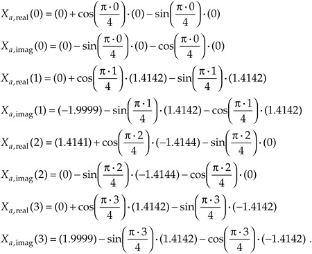
Evaluating the sine and cosine terms in Eq. (13-44),

Equation 13-45

Combining the results of the terms in Eq. (13-45), we have our final correct answer of

Equation 13-46

After going through all the steps required by Eqs. (13-35) through (13-40), the reader might question the efficiency of this 2N-Point Real FFT algorithm. Using the same process as the above Two N-Point Real FFTs algorithm analysis, let's show that the 2N-Point Real FFT algorithm does provide some modest computational saving. First, we know that a single 2N-Point radix-2 FFT has (2N/2) · log22N = N · (log2N+1) butterflies and requires

Equation 13-47

and

Equation 13-47'

If we add up the number of real multiplications and real additions required by the algorithm's N-point complex FFT, plus those required by Eqs. (13-35) through (13-38) and those required by Eqs. (13-39) and (13-40), the complete 2N-Point Real FFT algorithm requires

Equation 13-48

and

Equation 13-48'

OK, using the same hardware considerations (multiplications only) we used to arrive at Eq. (13-32), the percentage gain in multiplication saving of the 2N-Point Real FFT algorithm relative to a 2N-point complex FFT is

Equation 13-49

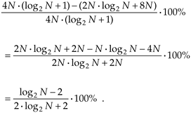
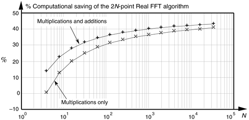
The computational (multiplications only) saving from Eq. (13-49) is plotted as the bottom curve of Figure 13-13. In terms of multiplications, the 2N-Point Real FFT algorithm provides a saving of >30% when N 128 or whenever we transform input data sequences whose lengths are 256.

Figure 13-13. Computational saving of the 2N-Point Real FFT algorithm over that of a single 2N-point complex FFT. The top curve is the saving when both additions and multiplications are used in the comparison. The bottom curve indicates the saving when only multiplications are considered.

Again, for hardware using high-speed multipliers, we consider both multiplication and addition operations. The difference between those combined arithmetic operations in Eqs. (13-47) plus (13-47') and Eqs. (13-48) plus (13-48') is the appropriate comparison. In this case, the percentage gain in computational saving of our algorithm is

Equation 13-50