DISCRETE LINEAR SYSTEMS | Chapter One. Discrete Sequences and Systems

The term linear defines a special class of systems where the output is the superposition, or sum, of the individual outputs had the individual inputs been applied separately to the system. For example, we can say that the application of an input x1(n) to a system results in an output y1(n). We symbolize this situation with the following expression:

Given a different input x2(n), the system has a y2(n) output as

Equation 1-12

For the system to be linear, when its input is the sum x1(n) + x2(n), its output must be the sum of the individual outputs so that

Equation 1-13

One way to paraphrase expression (1-13) is to state that a linear system's output is the sum of the outputs of its parts. Also, part of this description of linearity is a proportionality characteristic. This means that if the inputs are scaled by constant factors c1 and c2 then the output sequence parts are also scaled by those factors as

Equation 1-14

In the literature, this proportionality attribute of linear systems in expression (1-14) is sometimes called the homogeneity property. With these thoughts in mind, then, let's demonstrate the concept of system linearity.

1.5.1 Example of a Linear System

To illustrate system linearity, let's say we have the discrete system shown in Figure 1-7(a) whose output is defined as

Equation 1-15

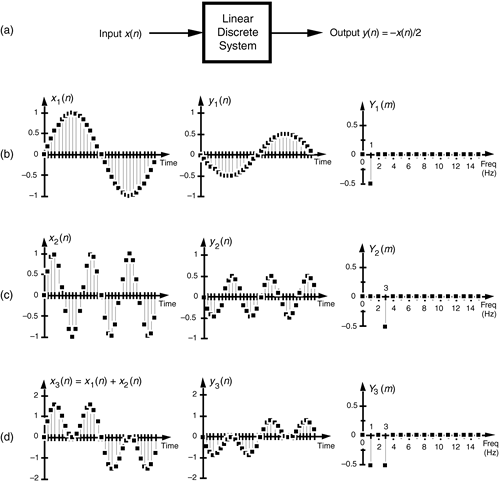
Figure 1-7. Linear system input-to-output relationships: (a) system block diagram where y(n) = –x(n)/2; (b) system input and output with a 1-Hz sinewave applied; (c) with a 3-Hz sinewave applied; (d) with the sum of 1-Hz and 3-Hz sinewaves applied.

that is, the output sequence is equal to the negative of the input sequence with the amplitude reduced by a factor of two. If we apply an x1(n) input sequence representing a 1-Hz sinewave sampled at a rate of 32 samples per cycle, we'll have a y1(n) output as shown in the center of Figure 1-7(b). The frequency-domain spectral amplitude of the y1(n) output is the plot on the right side of Figure 1-7(b), indicating that the output comprises a single tone of peak amplitude equal to –0.5 whose frequency is 1 Hz. Next, applying an x2(n) input sequence representing a 3-Hz sinewave, the system provides a y2(n) output sequence, as shown in the center of Figure 1-7(c). The spectrum of the y2(n) output, Y2(m), confirming a single 3-Hz sinewave output is shown on the right side of Figure 1-7(c). Finally—here's where the linearity comes in—if we apply an x3(n) input sequence that's the sum of a 1-Hz sinewave and a 3-Hz sinewave, the y3(n) output is as shown in the center of Figure 1-7(d). Notice how y3(n) is the sample-for-sample sum of y1(n) and y2(n). Figure 1-7(d) also shows that the output spectrum Y3(m) is the sum of Y1(m) and Y2(m). That's linearity.

1.5.2 Example of a Nonlinear System

It's easy to demonstrate how a nonlinear system yields an output that is not equal to the sum of y1(n) and y2(n) when its input is x1(n) + x2(n). A simple example of a nonlinear discrete system is that in Figure 1-8(a) where the output is the square of the input described by

Equation 1-16

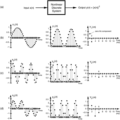
Figure 1-8. Nonlinear system input-to-output relationships: (a) system block diagram where y(n) = [x(n)]2; (b) system input and output with a 1-Hz sinewave applied; (c) with a 3-Hz sinewave applied; (d) with the sum of 1-Hz and 3-Hz sinewaves applied.

We'll use a well known trigonometric identity and a little algebra to predict the output of this nonlinear system when the input comprises simple sinewaves. Following the form of Eq. (1-3), let's describe a sinusoidal sequence, whose frequency fo = 1 Hz, by

Equation 1-17

Equation (1-17) describes the x1(n) sequence on the left side of Figure 1-8(b). Given this x1(n) input sequence, the y1(n) output of the nonlinear system is the square of a 1-Hz sinewave, or

Equation 1-18

We can simplify our expression for y1(n) in Eq. (1-18) by using the following trigonometric identity:

Equation 1-19

Using Eq. (1-19), we can express y1(n) as

Equation 1-20

which is shown as the all positive sequence in the center of Figure 1-8(b). Because Eq. (1-19) results in a frequency sum (a + b) and frequency difference (a – b) effect when multiplying two sinusoids, the y1(n) output sequence will be a cosine wave of 2 Hz and a peak amplitude of –0.5, added to a constant value of 1/2. The constant value of 1/2 in Eq. (1-20) is interpreted as a zero Hz frequency component, as shown in the Y1(m) spectrum in Figure 1-8(b). We could go through the same algebraic exercise to determine that, when a 3-Hz sinewave x2(n) sequence is applied to this nonlinear system, the output y2(n) would contain a zero Hz component and a 6 Hz component, as shown in Figure 1-8(c).

System nonlinearity is evident if we apply an x3(n) sequence comprising the sum of a 1-Hz and a 3-Hz sinewave as shown in Figure 1-8(d). We can predict the frequency content of the y3(n) output sequence by using the algebraic relationship

Equation 1-21

where a and b represent the 1-Hz and 3-Hz sinewaves, respectively. From Eq. (1-19), the a2 term in Eq. (1-21) generates the zero-Hz and 2-Hz output sinusoids in Figure 1-8(b). Likewise, the b2 term produces in y3(n) another zero-Hz and the 6-Hz sinusoid in Figure 1-8(c). However, the 2ab term yields additional 2-Hz and 4-Hz sinusoids in y3(n). We can show this algebraically by using Eq. (1-19) and expressing the 2ab term in Eq. (1-21) as

Equation 1-22

Equation (1-22) tells us that two additional sinusoidal components will be present in y3(n) because of the system's nonlinearity, a 2-Hz cosine wave whose amplitude is +1 and a 4-Hz cosine wave having an amplitude of –1. These spectral components are illustrated in Y3(m) on the right side of Figure 1-8(d).

Notice that, when the sum of the two sinewaves is applied to the nonlinear system, the output contained sinusoids, Eq. (1-22), that were not present in either of the outputs when the individual sinewaves alone were applied. Those extra sinusoids were generated by an interaction of the two input sinusoids due to the squaring operation. That's nonlinearity; expression (1-13) was not satisfied. (Electrical engineers recognize this effect of internally generated sinusoids as intermodulation distortion.) Although nonlinear systems are usually difficult to analyze, they are occasionally used in practice. References [2], [3], and [4], for example, describe their application in nonlinear digital filters. Again, expressions (1-13) and (1-14) state that a linear system's output resulting from a sum of individual inputs, is the superposition (sum) of the individual outputs. They also stipulate that the output sequence y1(n) depends only on x1(n) combined with the system characteristics, and not on the other input x2(n), i.e., there's no interaction between inputs x1(n) and x2(n) at the output of a linear system.

The first term in Eq. (1-22) is cos(2p · nts – 6p · nts) = cos(–4p · nts) = cos(–2p · 2 · nts). However, because the cosine function is even, cos(–a) = cos(a), we can express that first term as cos(2p · 2 · nts).