ALIASING: SIGNAL AMBIGUITY IN THE FREQUENCY DOMAIN

Table of contents:

ALIASING SIGNAL AMBIGUITY IN THE FREQUENCY DOMAIN

ALIASING SIGNAL AMBIGUITY IN THE FREQUENCY DOMAIN

There is a frequency-domain ambiguity associated with discrete-time signal samples that does not exist in the continuous signal world, and we can appreciate the effects of this uncertainty by understanding the sampled nature of discrete data. By way of example, suppose you were given the following sequence of values,

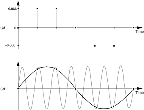
and were told that they represent instantaneous values of a time-domain sinewave taken at periodic intervals. Next, you were asked to draw that sinewave. You'd start by plotting the sequence of values shown by the dots in Figure 2-1(a). Next, you'd be likely to draw the sinewave, illustrated by the solid line in Figure 2-1(b), that passes through the points representing the original sequence.

Figure 2-1. Frequency ambiguity: (a) discrete-time sequence of values; (b) two different sinewaves that pass through the points of the discrete sequence.

Another person, however, might draw the sinewave shown by the shaded line in Figure 2-1(b). We see that the original sequence of values could, with equal validity, represent sampled values of both sinewaves. The key issue is that, if the data sequence represented periodic samples of a sinewave, we cannot unambiguously determine the frequency of the sinewave from those sample values alone.

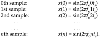
Reviewing the mathematical origin of this frequency ambiguity enables us not only to deal with it, but to use it to our advantage. Let's derive an expression for this frequency-domain ambiguity and, then, look at a few specific examples. Consider the continuous time-domain sinusoidal signal defined as

This x(t) signal is a garden variety sinewave whose frequency is fo Hz. Now let's sample x(t) at a rate of fs samples/s, i.e., at regular periods of ts seconds where ts = 1/fs. If we start sampling at time t = 0, we will obtain samples at times 0ts, 1ts, 2ts, and so on. So, from Eq. (2-1), the first n successive samples have the values

Equation 2-2

Equation (2-2) defines the value of the nth sample of our x(n) sequence to be equal to the original sinewave at the time instant nts. Because two values of a sinewave are identical if they're separated by an integer multiple of 2p radians, i.e., sin(ø) = sin(ø+2pm) where m is any integer, we can modify Eq. (2-2) as

Equation 2-3

If we let m be an integer multiple of n, m = kn, we can replace the m/n ratio in Eq. (2-3) with k so that

Equation 2-4

Because fs = 1/ts, we can equate the x(n) sequences in Eqs. (2-2) and (2-4) as

Equation 2-5

The fo and (fo+kfs) factors in Eq. (2-5) are therefore equal. The implication of Eq. (2-5) is critical. It means that an x(n) sequence of digital sample values, representing a sinewave of fo Hz, also exactly represents sinewaves at other frequencies, namely, fo + kfs. This is one of the most important relationships in the field of digital signal processing. It's the thread with which all sampling schemes are woven. In words, Eq. (2-5) states that

When sampling at a rate of fs samples/s, if k is any positive or negative integer, we cannot distinguish between the sampled values of a sinewave of fo Hz and a sinewave of (fo+kfs) Hz.

It's true. No sequence of values stored in a computer, for example, can unambiguously represent one and only one sinusoid without additional information. This fact applies equally to A/D-converter output samples as well as signal samples generated by computer software routines. The sampled nature of any sequence of discrete values makes that sequence also represent an infinite number of different sinusoids.

Equation (2-5) influences all digital signal processing schemes. It's the reason that, although we've only shown it for sinewaves, we'll see in Chapter 3 that the spectrum of any discrete series of sampled values contains periodic replications of the original continuous spectrum. The period between these replicated spectra in the frequency domain will always be fs, and the spectral replications repeat all the way from DC to daylight in both directions of the frequency spectrum. That's because k in Eq. (2-5) can be any positive or negative integer. (In Chapters 5 and 6, we'll learn that Eq. (2-5) is the reason that all digital filter frequency responses are periodic in the frequency domain and is crucial to analyzing and designing a popular type of digital filter known as the infinite impulse response filter.)

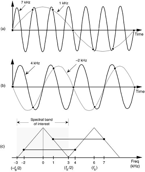
To illustrate the effects of Eq. (2-5), let's build on Figure 2-1 and consider the sampling of a 7-kHz sinewave at a sample rate of 6 kHz. A new sample is determined every 1/6000 seconds, or once every 167 microseconds, and their values are shown as the dots in Figure 2-2(a).

Figure 2-2. Frequency ambiguity effects of Eq. (2-5): (a) sampling a 7-kHz sinewave at a sample rate of 6 kHz; (b) sampling a 4-kHz sinewave at a sample rate of 6 kHz; (c) spectral relationships showing aliasing of the 7- and 4-kHz sinewaves.

Notice that the sample values would not change at all if, instead, we were sampling a 1-kHz sinewave. In this example fo = 7 kHz, fs = 6 kHz, and k = –1 in Eq. (2-5), such that fo+kfs = [7+(–1·6)] = 1 kHz. Our problem is that no processing scheme can determine if the sequence of sampled values, whose amplitudes are represented by the dots, came from a 7-kHz or a 1-kHz sinusoid. If these amplitude values are applied to a digital process that detects energy at 1 kHz, the detector output would indicate energy at 1 kHz. But we know that there is no 1-kHz tone there—our input is a spectrally pure 7-kHz tone. Equation (2-5) is causing a sinusoid, whose name is 7 kHz, to go by the alias of 1 kHz. Asking someone to determine which sinewave frequency accounts for the sample values in Figure 2-2(a) is like asking them "When I add two numbers I get a sum of four. What are the two numbers?" The answer is that there is an infinite number of number pairs that can add up to four.

Figure 2-2(b) shows another example of frequency ambiguity, that we'll call aliasing, where a 4-kHz sinewave could be mistaken for a –2-kHz sinewave. In Figure 2-2(b), fo = 4 kHz, fs = 6 kHz, and k = –1 in Eq. (2-5), so that fo+kfs = [4+(–1 · 6)] = –2 kHz. Again, if we examine a sequence of numbers representing the dots in Figure 2-2(b), we could not determine if the sampled sinewave was a 4-kHz tone or a –2-kHz tone. (Although the concept of negative frequencies might seem a bit strange, it provides a beautifully consistent methodology for predicting the spectral effects of sampling. Chapter 8 discusses negative frequencies and how they relate to real and complex signals.)

Now, if we restrict our spectral band of interest to the frequency range of ±fs/2 Hz, the previous two examples take on a special significance. The frequency fs/2 is an important quantity in sampling theory and is referred to by different names in the literature, such as critical Nyquist, half Nyquist, and folding frequency. A graphical depiction of our two frequency aliasing examples is provided in Figure 2-2(c). We're interested in signal components that are aliased into the frequency band between –fs/2 and +fs/2. Notice in Figure 2-2(c) that, within the spectral band of interest (±3 kHz, because fs = 6 kHz), there is energy at –2 kHz and +1 kHz, aliased from 4 kHz and 7 kHz, respectively. Note also that the vertical positions of the dots in Figure 2-2(c) have no amplitude significance but that their horizontal positions indicate which frequencies are related through aliasing.

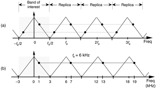
A general illustration of aliasing is provided in the shark's tooth pattern in Figure 2-3(a). Note how the peaks of the pattern are located at integer multiples of fs Hz. The pattern shows how signals residing at the intersection of a horizontal line and a sloped line will be aliased to all of the intersections of that horizontal line and all other lines with like slopes. For example, the pattern in Figure 2-3(b) shows that our sampling of a 7-kHz sinewave at a sample rate of 6 kHz will provide a discrete sequence of numbers whose spectrum ambiguously represents tones at 1 kHz, 7 kHz, 13 kHz, 19 kHz, etc. Let's pause for a moment and let these very important concepts soak in a bit. Again, discrete sequence representations of a continuous signal have unavoidable ambiguities in their frequency domains. These ambiguities must be taken into account in all practical digital signal processing algorithms.

Figure 2-3. Shark's tooth pattern: (a) aliasing at multiples of the sampling frequency; (b) aliasing of the 7-kHz sinewave to 1 kHz, 13 kHz, and 19 kHz.