INTERPOLATION
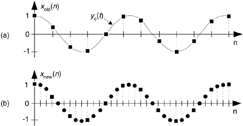
As we said before, decimation is only part of the sample rate conversion story—now let's consider interpolation. Sample rate increase by interpolation is a bit more involved than decimation because with interpolation, new sample values need to be calculated. Conceptually, interpolation comprises the generation of a continuous yc(t) curve passing through our xold(n) sampled values, as shown in Figure 10-5(a), followed by sampling that curve at the new sample rate fnew to obtain the interpolated sequence xnew(n) in Figure 10-5(b). Of course, continuous curves can't exist inside a digital machine, so we'll just have to obtain xnew(n) directly from xold(n). To increase a given sample rate, or upsample, by a factor of M, we have to calculate M-1 intermediate values between each sample in xold(n). The process is beautifully straightforward and best understood by way of an example.
Figure 10-5. Sample rate conversion: (a) original sequence; (b) interpolated by three sequence.

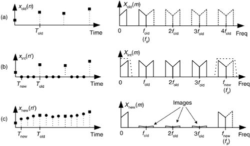
Let's assume we have the sequence xold(n), part of which is shown in Figure 10-6(a), and we want to increase its sample rate by a factor of M = 4. The xold(n) sequence's spectrum is provided in Figure 10-6(a), where the signal spectrum between zero Hz and 4fold is shown. Please notice: the dashed curves in Xold(m) are spectral replications. To upsample xold(n) by a factor of four, we typically insert three zeros between each sample, as shown in Figure 10-6(b) to create the new sequence xint(n'). The 'int' subscript means intermediate. Notice xint(n') = xold(n), when n' = 4n. That is, the old sequence is now embedded in the new sequence. The insertion of the zeros (a process called zero stuffing) establishes the sample index for the new sequence xint(n') where the interpolated values will be assigned.
Figure 10-6. Interpolation by a factor of four: (a) original sampled sequence and its spectrum; (b) zeros inserted in original sequence and resulting spectrum; (c) output sequence of interpolation filter and final interpolated spectrum.

The spectrum of xint(n'), Xint(m), is shown in Figure 10-6(b) where fnew = 4fold. The solid curves in Xint(m), centered at multiples of fold, are called images. What we've done by adding the zeros is merely increase the effective sample frequency to fs = fnew in Figure 10-6(b). The final step in interpolation is to filter the xint(n') sequence with a lowpass digital filter, whose frequency response is shown as the dashed lines about zero Hz and fnew Hz, in Figure 10-6(b), to attenuate the spectral images. This lowpass filter is called an interpolation filter, and its output sequence is the desired xnew(n') in Figure 10-6(c) having the spectrum Xnew(m).
Is that all there is to zero stuffing, interpolation, and filtering? Well, not quite—because we can't implement an ideal lowpass filter, xnew(n') will not be an exact interpolation of xold(n). The error manifests itself as the residual images within Xnew(m). With an ideal filter, these images would not exist. We can only approximate an ideal lowpass interpolation filter. The issue to remember is that the accuracy of our entire interpolation process depends on the stopband attenuation of our lowpass interpolation filter. The lower the attenuation, the more accurate the interpolation. As with decimation, interpolation can be thought of as an exercise in lowpass filter design.
Note that the interpolation process, because of the zero-valued samples, has an inherent amplitude loss factor of M. Thus to achieve unity gain between sequences xold(n) and xnew(n'), the interpolation filter must have a gain of M.
One last issue regarding interpolation. You might fall into the trap of thinking interpolation was born of modern-day signal processing activities (for example, when we interpolate/upsample a music signal before applying it to a digital-to-analog (D/A) converter for routing to an amplifier and speaker in compact disk players. That upsampling reduces the cost of the analog filter following the D/A converter). Please don't. Ancient astronomical cuneiform tablets (originating in Uruk and Babylon 200 years before the birth of Jesus) indicate linear interpolation was used to fill in the missing tabulated positions of celestial bodies for those times when atmospheric conditions prevented direct observation[3]. Interpolation has been used ever since, for filling in missing data.
 |
Amazon |  |
