UNDERSTANDING THE DFT EQUATION
Equation (3-2) has a tangled, almost unfriendly, look about it. Not to worry. After studying this chapter, Eq. (3-2) will become one of our most familiar and powerful tools in understanding digital signal processing. Let's get started by expressing Eq. (3-2) in a different way and examining it carefully. From Euler's relationship e–jø = cos(ø) –jsin(ø), Eq. (3-2) is equivalent to
We have separated the complex exponential of Eq. (3-2) into its real and imaginary components where
|
X(m) |
= |
the mth DFT output component, i.e., X(0), X(1), X(2), X(3), etc., |
|
m |
= |
the index of the DFT output in the frequency domain, |
|
m |
= |
0, 1, 2, 3, . . ., N–1, |
|
x(n) |
= |
the sequence of input samples, x(0), x(1), x(2), x(3), etc., |
|
n |
= |
the time-domain index of the input samples, n = 0, 1, 2, 3, . . ., N–1, |
|
j |
= |
|
|
N |
= |
the number of samples of the input sequence and the number of frequency points in the DFT output. |
Although it looks more complicated than Eq. (3-2), Eq. (3-3) turns out to be easier to understand. (If you're not too comfortable with it, don't let the j =  concept bother you too much. It's merely a convenient abstraction that helps us compare the phase relationship between various sinusoidal components of a signal. Chapter 8 discusses the j operator in some detail.)[] The indices for the input samples (n) and the DFT output samples (m) always go from 0 to N–1 in the standard DFT notation. This means that with N input time-domain sample values, the DFT determines the spectral content of the input at N equally spaced frequency points. The value N is an important parameter because it determines how many input samples are needed, the resolution of the frequency-domain results, and the amount of processing time necessary to calculate an N-point DFT.
[] Instead of the letter j, be aware that mathematicians often use the letter i to represent the
It's useful to see the structure of Eq. (3-3) by eliminating the summation and writing out all the terms. For example, when N = 4, n and m both go from 0 to 3, and Eq. (3-3) becomes
Equation 3-4a
Writing out all the terms for the first DFT output term corresponding to m = 0,
Equation 3-4b
For the second DFT output term corresponding to m = 1, Eq. (3-4a) becomes
Equation 3-4c

For the third output term corresponding to m = 2, Eq. (3-4a) becomes
Equation 3-4d
Finally, for the fourth and last output term corresponding to m = 3, Eq. (3-4a) becomes
Equation 3-4e
The above multiplication symbol "·" in Eq. (3-4) is used merely to separate the factors in the sine and cosine terms. The pattern in Eq. (3-4b) through (3-4e) is apparent now, and we can certainly see why it's convenient to use the summation sign in Eq. (3-3). Each X(m) DFT output term is the sum of the point for point product between an input sequence of signal values and a complex sinusoid of the form cos(ø) – jsin(ø). The exact frequencies of the different sinusoids depend on both the sampling rate fs, at which the original signal was sampled, and the number of samples N. For example, if we are sampling a continuous signal at a rate of 500 samples/s and, then, perform a 16-point DFT on the sampled data, the fundamental frequency of the sinusoids is fs/N = 500/16 or 31.25 Hz. The other X(m) analysis frequencies are integral multiples of the fundamental frequency, i.e.,
|
X(0) |
= |
1st frequency term, with analysis frequency = 0 · 31.25 = 0 Hz, |
|
X(1) |
= |
2nd frequency term, with analysis frequency = 1 · 31.25 = 31.25 Hz, |
|
X(2) |
= |
3rd frequency term, with analysis frequency = 2 · 31.25 = 62.5 Hz, |
|
X(3) |
= |
4th frequency term, with analysis frequency = 3 · 31.25 = 93.75 Hz, |
|
. . . |
||
|
. . . |
||
|
X(15) |
= |
16th frequency term, with analysis frequency = 15 · 31.25 = 468.75 Hz. |
The N separate DFT analysis frequencies are
Equation 3-5
So, in this example, the X(0) DFT term tells us the magnitude of any 0-Hz ("DC") component contained in the input signal, the X(1) term specifies the magnitude of any 31.25-Hz component in the input signal, and the X(2) term indicates the magnitude of any 62.5-Hz component in the input signal, etc. Moreover, as we'll soon show by example, the DFT output terms also determine the phase relationship between the various analysis frequencies contained in an input signal.
Quite often we're interested in both the magnitude and the power (magnitude squared) contained in each X(m) term, and the standard definitions for right triangles apply here as depicted in Figure 3-1.
Figure 3-1. Trigonometric relationships of an individual DFT X(m) complex output value.
If we represent an arbitrary DFT output value, X(m), by its real and imaginary parts
Equation 3-6

the magnitude of X(m) is
Equation 3-7

By definition, the phase angle of X(m), Xø(m), is
Equation 3-8
The power of X(m), referred to as the power spectrum, is the magnitude squared where
Equation 3-9

3.1.1 DFT Example 1
The above Eqs. (3-2) and (3-3) will become more meaningful by way of an example, so, let's go through a simple one step-by-step. Let's say we want to sample and perform an 8-point DFT on a continuous input signal containing components at 1 kHz and 2 kHz, expressed as
Equation 3-10

To make our example input signal xin(t) a little more interesting, we have the 2-kHz term shifted in phase by 135° (3p/4 radians) relative to the 1-kHz sinewave. With a sample rate of fs, we sample the input every 1/fs = ts seconds. Because N = 8, we need 8 input sample values on which to perform the DFT. So the 8-element sequence x(n) is equal to xin(t) sampled at the nts instants in time so that
Equation 3-11

If we choose to sample xin(t) at a rate of fs = 8000 samples/s from Eq. (3-5), our DFT results will indicate what signal amplitude exists in x(n) at the analysis frequencies of mfs/N, or 0 kHz, 1 kHz, 2 kHz, . . ., 7 kHz. With fs = 8000 samples/s, our eight x(n) samples are
Equation 3-11'
These x(n) sample values are the dots plotted on the solid continuous xin(t) curve in Figure 3-2(a). (Note that the sum of the sinusoidal terms in Eq. (3-10), shown as the dashed curves in Figure 3-2(a), is equal to xin(t).)
Figure 3-2. DFT Example 1: (a) the input signal; (b) the input signal and the m = 1 sinusoids; (c) the input signal and the m = 2 sinusoids; (d) the input signal and the m = 3 sinusoids.
Now we're ready to apply Eq. (3-3) to determine the DFT of our x(n) input. We'll start with m = 1 because the m = 0 case leads to a special result that we'll discuss shortly. So, for m = 1, or the 1-kHz (mfs/N = 1·8000/8) DFT frequency term, Eq. (3-3) for this example becomes
Equation 3-12
Next we multiply x(n) by successive points on the cosine and sine curves of the first analysis frequency that have a single cycle over our 8 input samples. In our example, for m = 1, we'll sum the products of the x(n) sequence with a 1-kHz cosine wave and a 1-kHz sinewave evaluated at the angular values of 2pn/8. Those analysis sinusoids are shown as the dashed curves in Figure 3-2(b). Notice how the cosine and sinewaves have m = 1 complete cycles in our sample interval.
Substituting our x(n) sample values into Eq. (3-12) and listing the cosine terms in the left column and the sine terms in the right column, we have
|
X(1) |
= 0.3535 · 1.0 |
– j(0.3535 · 0.0) |
|
||
|
+ 0.3535 · 0.707 |
– j(0.3535 · 0.707) |
|
|||
|
+ 0.6464 · 0.0 |
– j(0.6464 · 1.0) |
|
|||
|
+ 1.0607 · –0.707 |
– j(1.0607 · 0.707) |
. . . |
|||
|
+ 0.3535 · –1.0 |
– j(0.3535 · 0.0) |
. . . |
|||
|
– 1.0607 · –0.707 |
– j(–1.0607 · –0.707) |
. . . |
|||
|
– 1.3535 · 0.0 |
– j(–1.3535 · –1.0) |
. . . |
|||
|
– 0.3535 · 0.707 |
– j(–0.3535 · –0.707) |
|
|||
|
= |
0.3535 |
+ j0.0 |
|||
|
+ 0.250 |
– j0.250 |
||||
|
+ 0.0 |
– j0.6464 |
||||
|
– 0.750 |
– j0.750 |
||||
|
– 0.3535 |
– j0.0 |
||||
|
+ 0.750 |
– j0.750 |
||||
|
+ 0.0 |
– j1.3535 |
||||
|
– 0.250 |
– j0.250 |
||||
|
= |
0.0 – j4.0 = 4 |
||||
 this is the n = 0 term
 –90°.
–90°.So we now see that the input x(n) contains a signal component at a frequency of 1 kHz. Using Eq. (3-7), Eq. (3-8), and Eq. (3-9) for our X(1) result, Xmag(1) = 4, XPS(1) = 16, and X(1)'s phase angle relative to a 1-kHz cosine is Xø(1) = –90°.
For the m = 2 frequency term, we correlate x(n) with a 2-kHz cosine wave and a 2-kHz sinewave. These waves are the dashed curves in Figure 3-2(c). Notice here that the cosine and sinewaves have m = 2 complete cycles in our sample interval in Figure 3-2(c). Substituting our x(n) sample values in Eq. (3-3), for m = 2, gives
|
X(2) |
= 0.3535 · 1.0 |
– j(0.3535 · 0.0) |
|||
|
+ 0.3535 · 0.0 |
– j(0.3535 · 1.0) |
||||
|
+ 0.6464 · –1.0 |
– j(0.6464 · 0.0) |
||||
|
+ 1.0607 · 0.0 |
– j(1.0607 · –1.0) |
||||
|
+ 0.3535 · 1.0 |
– j(0.3535 · 0.0) |
||||
|
–1.0607 · 0.0 |
– j(–1.0607 · 1.0) |
||||
|
–1.3535 · –1.0 |
– j(–1.3535 · 0.0) |
||||
|
–0.3535 · 0.0 |
– j(–0.3535 · –1.0) |
||||
|
= |
0.3535 |
+ j0.0 |
|||
|
+ 0.0 |
– j0.3535 |
||||
|
– 0.6464 |
– j0.0 |
||||
|
– 0.0 |
+ j1.0607 |
||||
|
+ 0.3535 |
– j0.0 |
||||
|
+ 0.0 |
+ j1.0607 |
||||
|
+ 1.3535 |
– j0.0 |
||||
|
– 0.0 |
– j0.3535 |
||||
|
= |
1.414 + j1.414 = 2 |
||||
Here our input x(n) contains a signal at a frequency of 2 kHz whose relative amplitude is 2, and whose phase angle relative to a 2-kHz cosine is 45°. For the m = 3 frequency term, we correlate x(n) with a 3-kHz cosine wave and a 3-kHz sinewave. These waves are the dashed curves in Figure 3-2(d). Again, see how the cosine and sinewaves have m = 3 complete cycles in our sample interval in Figure 3-2(d). Substituting our x(n) sample values in Eq. (3-3) for m = 3 gives
|
X(3) |
= 0.3535 · 1.0 |
– j(0.3535 · 0.0) |
||
|
+ 0.3535 · –0.707 |
– j(0.3535 · 0.707) |
|||
|
+ 0.6464 · 0.0 |
– j(0.6464 · –1.0) |
|||
|
+ 1.0607 · 0.707 |
– j(1.0607 · 0.707) |
|||
|
+ 0.3535 · –1.0 |
– j(0.3535 · 0.0) |
|||
|
– 1.0607 · 0.707 |
– j(–1.0607 · –0.707) |
|||
|
– 1.3535 · 0.0 |
– j(–1.3535 · 1.0) |
|||
|
– 0.3535 · –0.707 |
– j(–0.3535 · –0.707) |
|||
|
= |
0.3535 |
+ j0.0 |
||
|
– 0.250 |
– j0.250 |
|||
|
+ 0.0 |
+ j0.6464 |
|||
|
+ 0.750 |
– j0.750 |
|||
|
– 0.3535 |
– j0.0 |
|||
|
– 0.750 |
– j0.750 |
|||
|
+ 0.0 |
+ j1.3535 |
|||
|
+ 0.250 |
– j0.250 |
|||
|
= |
0.0 – j0.0 = 0 |
|||
Our DFT indicates that x(n) contained no signal at a frequency of 3 kHz. Let's continue our DFT for the m = 4 frequency term using the sinusoids in Figure 3-3(a).
Figure 3-3. DFT Example 1: (a) the input signal and the m = 4 sinusoids; (b) the input and the m = 5 sinusoids; (c) the input and the m = 6 sinusoids; (d) the input and the m = 7 sinusoids.
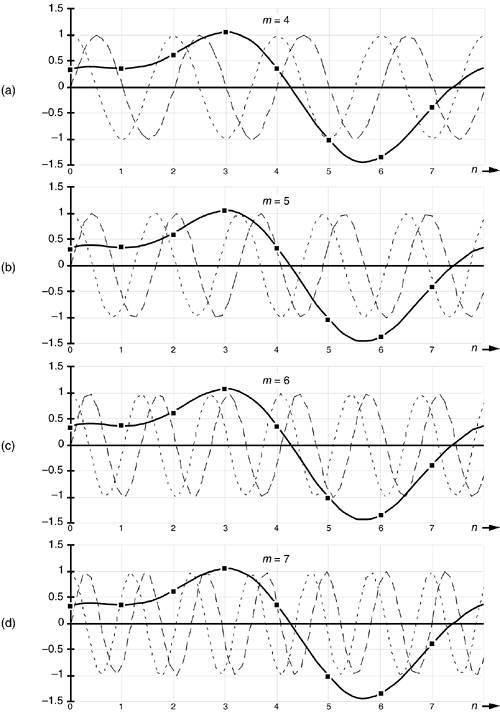
So Eq. (3-3) is
|
X(4) |
= 0.3535 · 1.0 |
– j(0.3535 · 0.0) |
||
|
+ 0.3535 · –1.0 |
– j(0.3535 · 0.0) |
|||
|
+ 0.6464 · 1.0 |
– j(0.6464 · 0.0) |
|||
|
+ 1.0607 · –1.0 |
– j(1.0607 · 0.0) |
|||
|
+ 0.3535 · 1.0 |
– j(0.3535 · 0.0) |
|||
|
– 1.0607 · –1.0 |
– j(–1.0607 · 0.0) |
|||
|
– 1.3535 · 1.0 |
– j(–1.3535 · 0.0) |
|||
|
– 0.3535 · –1.0 |
– j(–0.3535 · 0.0) |
|||
|
= |
0.3535 |
– j0.0 |
||
|
– 0.3535 |
– j0.0 |
|||
|
+ 0.6464 |
– j0.0 |
|||
|
– 1.0607 |
– j0.0 |
|||
|
+ 0.3535 |
– j0.0 |
|||
|
+ 1.0607 |
– j0.0 |
|||
|
– 1.3535 |
– j0.0 |
|||
|
+ 0.3535 |
– j0.0 |
|||
|
= |
0.0 – j0.0 = 0 |
|||
Our DFT for the m = 5 frequency term using the sinusoids in Figure 3-3(b) yields
|
X(5) |
= 0.3535 · 1.0 |
– j(0.3535 · 0.0) |
||
|
+ 0.3535 · –0.707 |
– j(0.3535 · –0.707) |
|||
|
+ 0.6464 · 0.0 |
– j(0.6464 · 1.0) |
|||
|
+ 1.0607 · 0.707 |
– j(1.0607 · –0.707) |
|||
|
+ 0.3535 · –1.0 |
– j(0.3535 · 0.0) |
|||
|
– 1.0607 · 0.707 |
– j(–1.0607 · 0.707) |
|||
|
– 1.3535 · 0.0 |
– j(–1.3535 · –1.0) |
|||
|
– 0.3535 · –0.707 |
– j(–0.3535 · 0.707) |
|||
|
= |
0.3535 |
– j0.0 |
||
|
– 0.250 |
+ j0.250 |
|||
|
+ 0.0 |
– j0.6464 |
|||
|
+ 0.750 |
+ j0.750 |
|||
|
– 0.3535 |
– j0.0 |
|||
|
– 0.750 |
+ j0.750 |
|||
|
+ 0.0 |
– j1.3535 |
|||
|
+ 0.250 |
+ j0.250 |
|||
|
= |
0.0 – j.0 = 0 |
|||
For the m = 6 frequency term using the sinusoids in Figure 3-3(c), Eq. (3-3) is
| Amazon | ||
