TIME-DOMAIN INTERPOLATION USING THE FFT | Chapter Thirteen. Digital Signal Processing Tricks

The thoughtful reader may have looked at the Section 13.27 FIR filter impulse response interpolation scheme, and wondered, "If we can interpolate time-domain impulse responses, we should be able to interpolate time-domain signals using the same frequency-domain zero stuffing method". This is true, and the above interpolation-by-M process applied to time signals is sometimes called exact interpolation—because its performance is equivalent to using an ideal, infinite-stopband attenuation, time-domain interpolation filter—and has made its way into DSP textbooks, journal articles, and classroom notes of famous DSP professors.

To establish our notation, lets say we compute the FFT of an N-point x(n) time sequence to produce its X(m) frequency-domain samples. Next, we stuff (M–1)N zeros in the middle of X(m) to yield the MN-length Xint(m) frequency samples, where MN is an integer power of two. Then we perform an MN-point inverse FFT on Xint(m) to obtain the interpolated-by-M xint(n) times samples. Using this frequency-domain zero stuffing to implement time-domain signal interpolation involves two important issues upon which we now focus.

13.28.1 Computing Interpolated Real Signals

The first issue: to ensure the interpolated xint(n) time sequence is real only, conjugate symmetry must be maintained in the zero-stuffed Xint(m) frequency samples. If the X(m) sequence has a nonzero sample at Xint(N/2), the fs/2 frequency component, we must use the following steps in computing Xint(m) to guarantee conjugate symmetry:

Perform an N-point FFT on an N-point x(n) time sequence, yielding N frequency samples, X(m).
Create an MN-point spectral sequence Xint(m) initially set to all zeros.
Assign Xint(m) = X(m), for 0 m (N/2)–1.
Assign both Xint(N/2) and Xint(MN–N/2) equal to X(N/2)/2. (This step, to maintain conjugate symmetry and improve interpolation accuracy, is not so well known[72].)
Assign Xint(m) = X(q), where MN–(N/2)+1 m MN–1, and (N/2)+1 q N–1.
Compute the MN-point inverse FFT of Xint(m) yielding the desired MN-length interpolated xint(n) sequence.
Finally, if desired, multiply xint(n) by M to compensate for the 1/M amplitude loss induced by interpolation.

Whew! Our mathematical notation makes this signal interpolation scheme look complicated, but it's really not so bad. Table 13-8 shows the frequency-domain Xint(m) sample assignments, where 0 m 15, to interpolate an N = 8-point x(n) sequence by a factor of M = 2.

One of the nice properties of the above algorithm is that every Mth xint(n) sample coincides with the original x(n) samples. In practice, due to our finite-precision computing, the imaginary parts of our final xint(n) may have small non-zero values. As such, we take xint(n) to the be real part of the inverse FFT of Xint(m).

Here's the second issue regarding time-domain real signal interpolation, and it's a big deal indeed. This exact interpolation algorithm provides correct results only if the original x(n) sequence is periodic within its full time interval. If X(m) exhibits any spectral leakage, like the signals with which we usually work, the interpolated xint(n) sequence can contain noticeable amplitude errors in its beginning and ending samples, as shown in Figure 13-74(a) where an N = 24 sample x(n) sequence is interpolated by M = 2. In that figure, squares (both white and black) represent the 48-point interpolated xint(n) sequence, white squares are the original x(n) samples, and circles represent the exactly correct interpolated sample values. (In the center portion of the figure, the circles are difficult to see because they're hidden behind the squares.) The interpolation error, the difference between the correct samples and xint(n), is given in Figure 13-74(b).

Figure 13-74. Interpolation results, N = 24, M = 2: (a) interpolated xint(n), original x(n), and correct interpolation; (b) interpolation error.

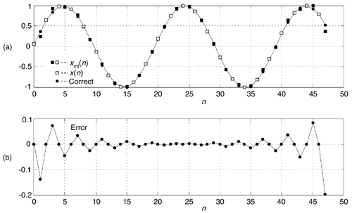
Table 13-8. XINT(m) Assignments for Interpolation by Two

m	Xint(m)	m	Xint(m)
0	X(0)	8	0
1	X(1)	9	_
2	X(2)	10	0
3	X(3)	11	0
4	X(4)/2	12	X(4)/2
5	0	13	X(5)
6	0	14	X(6)
7	0	15	X(7)

These interpolation errors exist because Xint(m) is not identical to the spectrum obtained had we sampled x(n) at a rate of Mfs and performed an MN-point forward FFT. There's no closed-form mathematical expression enabling us to predict these errors. The error depends on the spectral component magnitudes and phases within x(n), as well as N and M. Reference [72] reports a reduction in interpolation errors for two-dimensional image interpolation when, in an effort to reduce spectral leakage in X(m), simple windowing is applied to the first few and last few samples of x(n).

With the advent of fast hardware DSP chips and pipelined FFT techniques, the above time-domain interpolation algorithm may be viable for a number of applications, such as computing selectable sample rate time sequences of a test signal that has a fixed spectral envelope shape; providing interpolation, by selectable factors, of signals that were filtered in the frequency domain using the fast convolution method (Section 13.10); or digital image resampling. One scenario to consider is using the efficient 2N-Point Real FFT technique, described in Section 13.5.2, to compute the forward FFT of the real-valued x(n). Of course, the prudent engineer would conduct a literature search to see what algorithms are available for efficiently performing inverse FFTs when many of the frequency-domain samples are zeros.

13.28.2 Computing Interpolated Analytic Signals

We can use the frequency-domain zero stuffing scheme to generate an interpolated-by-M analytic time signal based upon the real N-point time sequence x(n), if N is even[73]. The process is as follows:

Perform an N-point FFT on an N-point real xr(n) time sequence, yielding N frequency samples, Xr(m).
Create an MN-point spectral sequence Xint(m) initially set to all zeros, where MN is an integer power of two.
Assign Xint(0) = Xr(0), and Xint(N/2) = Xr(N/2).
Assign Xint(m) = 2Xr(m), for 1 m = (N/2)–1.
Compute the MN-point inverse FFT of Xint(m) yielding the desired MN-length interpolated analytic (complex) xc,int(n) sequence.
Finally, if desired, multiply xc,int(n) by M to compensate for the 1/M amplitude loss induced by interpolation.