DFT SHIFTING THEOREM | Chapter Three. The Discrete Fourier Transform

There's an important property of the DFT known as the shifting theorem. It states that a shift in time of a periodic x(n) input sequence manifests itself as a constant phase shift in the angles associated with the DFT results. (We won't derive the shifting theorem equation here because its derivation is included in just about every digital signal processing textbook in print.) If we decide to sample x(n) starting at n equals some integer k, as opposed to n = 0, the DFT of those time-shifted sample values is Xshifted(m) where

Equation (3-19) tells us that, if the point where we start sampling x(n) is shifted to the right by k samples, the DFT output spectrum of Xshifted(m) is X(m) with each of X(m)'s complex terms multiplied by the linear phase shift ej2pkm/N, which is merely a phase shift of 2pkm/N radians or 360km/N degrees. Conversely, if the point where we start sampling x(n) is shifted to the left by k samples, the spectrum of Xshifted(m) is X(m) multiplied by e–j2pkm/N. Let's illustrate Eq. (3-19) with an example.

3.6.1 DFT Example 2

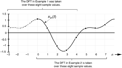
Suppose we sampled our DFT Example 1 input sequence later in time by k = 3 samples. Figure 3-5 shows the original input time function,

Figure 3-5. Comparison of sampling times between DFT Example 1 and DFT Example 2.

We can see that Figure 3-5 is a continuation of Figure 3-2(a). Our new x(n) sequence becomes the values represented by the solid black dots in Figure 3-5 whose values are

Equation 3-20

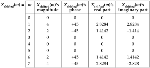
Performing the DFT on Eq. (3-20), Xshifted(m) is

Equation 3-21

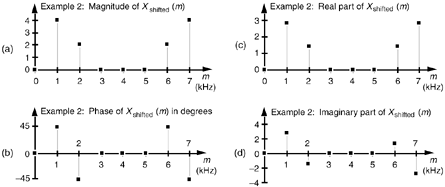
The values in Eq. (3-21) are illustrated as the dots in Figure 3-6. Notice that Figure 3-6(a) is identical to Figure 3-4(a). Equation (3-19) told us that the magnitude of Xshifted(m) should be unchanged from that of X(m). That's a comforting thought, isn't it? We wouldn't expect the DFT magnitude of our original periodic xin(t) to change just because we sampled it over a different time interval. The phase of the DFT result does, however, change depending on the instant at which we started to sample xin(t).

Figure 3-6. DFT results from Example 2: (a) magnitude of Xshifted(m); (b) phase of Xshifted(m); (c) real part of Xshifted(m); (d) imaginary part of Xshifted(m).

By looking at the m = 1 component of Xshifted(m), for example, we can double-check to see that phase values in Figure 3-6(b) are correct. Using Eq. (3-19) and remembering that X(1) from DFT Example 1 had a magnitude of 4 at a phase angle of –90 (or –p/2 radians), k = 3 and N = 8 so that

Equation 3-22