PHASE RESPONSE OF FIR FILTERS | Chapter Five. Finite Impulse Response Filters

Although we illustrated a couple of output phase shift examples for our original averaging FIR filter in Figure 5-10, the subject of FIR phase response deserves additional attention. One of the dominant features of FIR filters is their linear phase response that we can demonstrate by way of example. Given the 25 h(k) FIR filter coefficients in Figure 5-34(a), we can perform a DFT to determine the filter's H(m) frequency response. The normalized real part, imaginary part, and magnitude of H(m) are shown in Figures 5-34(b) and 5-34(c), respectively.[] Being complex values, each H(m) sample value can be described by its real and imaginary parts, or equivalently, by its magnitude |H(m)| and its phase Hø(m) shown in Figure 5-35(a).

[] Any DFT size greater than the h(k) width of 25 is sufficient to obtain H(m). The h(k) sequence was padded with 103 zeros to take a 128-point DFT resulting in the H(m) sample values in Figure 5-34.

Figure 5-34. FIR filter frequency response H(m): (a) h(k) filter coefficients; (b) real and imaginary parts of H(m); (c) magnitude of H(m).

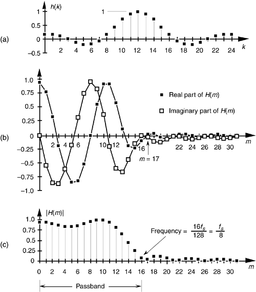
Figure 5-35. FIR filter phase response Hø(m) in degrees: (a) calculated Hø(m); (b) polar plot of Hø(m)'s first ten phase angles in degrees; (c) actual Hø(m).

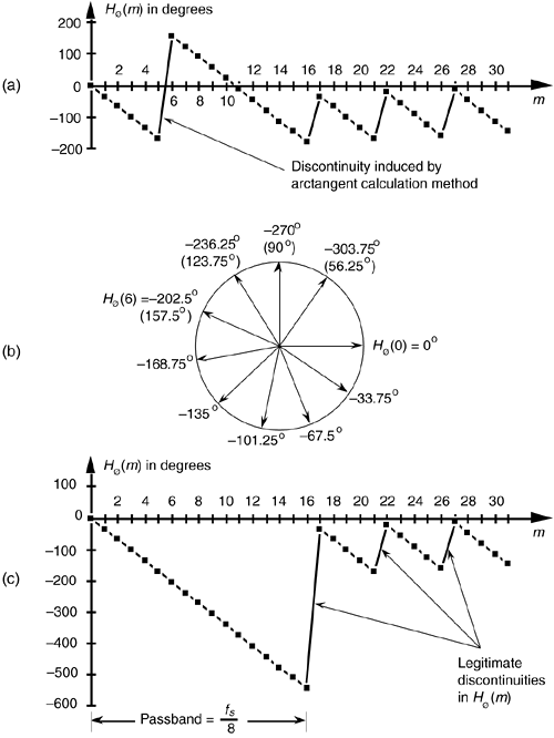
The phase of a complex quantity is, of course, the arctangent of the imaginary part divided by the real part, or ø = tan –1(imag/real). Thus the phase of Hø(m) is determined from the samples in Figure 5-34(b).

The phase response in Figure 5-35(a) certainly looks linear over selected frequency ranges, but what do we make of those sudden jumps, or discontinuities, in this phase response? If we were to plot the angles of Hø(m) starting with the m = 0 sample on a polar graph, using the nonzero real part of H(0), and the zero-valued imaginary part of H(0), we'd get the zero-angled Hø(0) phasor shown on the right side of Figure 5-35(b). Continuing to use the real and imaginary parts of H(m) to plot additional phase angles results in the phasors going clockwise around the circle in increments of –33.75°. It's at the Hø(6) that we discover the cause of the first discontinuity in Figure 5-35(a). Taking the real and imaginary parts of H(6), we'd plot our phasor oriented at an angle of –202.5°. But Figure 5-35(a) shows that Hø(6) is equal to 157.5°. The problem lies in the software routine used to generate the arctangent values plotted in Figure 5-35(a). The software adds 360° to any negative angles in the range of –180° > ø –360°, i.e., angles in the upper half of the circle. This makes ø a positive angle in the range of 0° < ø 180° and that's what gets plotted. (This apparent discontinuity between Hø(5) and Hø(6) is called phase wrapping.) So the true Hø(6) of –202.5° is converted to a +157.5° as shown in parentheses in Figure 5-35(b). If we continue our polar plot for additional Hø(m) values, we'll see that their phase angles continue to decrease with an angle increment of –33.75°. If we compensate for the software's behavior and plot phase angles more negative than –180°, by unwrapping the phase, we get the true Hø(m) shown in Figure 5-35(c).[] Notice that Hø(m) is, indeed, linear over the passband of H(m). It's at Hø(17) that our particular H(m) experiences a polarity change of its real part while its imaginary part remains negative—this induces a true phase angle discontinuity that really is a constituent of H(m) at m = 17. (Additional phase discontinuities occur each time the real part of H(m) reverses polarity, as shown in Figure 5-35(c).) The reader may wonder why we care about the linear phase response of H(m). The answer, an important one, requires us to introduce the notion of group delay.

[] When plotting filter phase responses, if we encounter a phase angle sample ø that looks like an unusual discontinuity, it's a good idea to add 360° to ø when ø is negative, or –360° when ø is positive, to see if that compensates for any software anomalies.

Group delay is defined as the negative of the derivative of the phase with respect to frequency, or G = –Dø/Df. For FIR filters, then, group delay is the slope of the Hø(m) response curve. When the group delay is constant, as it is over the passband of all FIR filters having symmetrical coefficients, all frequency components of the filter input signal are delayed by an equal amount of time G before they reach the filter's output. This means that no phase distortion is induced in the filter's desired output signal, and this is crucial in communications signals. For amplitude modulation (AM) signals, constant group delay preserves the time waveform shape of the signal's modulation envelope. That's important because the modulation portion of an AM signal contains the signal's information. Conversely, a nonlinear phase will distort the audio of AM broadcast signals, blur the edges of television video images, blunt the sharp edges of received radar pulses, and increase data errors in digital communication signals. (Group delay is sometimes called envelope delay because group delay was originally the subject of analysis due to its affect on the envelope, or modulation signal, of amplitude modulation AM systems.) Of course we're not really concerned with the group delay outside the passband because signal energy outside the passband is what we're trying to eliminate through filtering.

Over the passband frequency range for an S-tap FIR digital filter, group delay has been shown to be given by

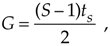
where ts is the sample period (1/fs).[] This group delay is measured in seconds. Eliminating, the ts factor in Eq. (5-23) would change its dimensions to samples. The value G, measured in samples, is always an integer for odd-tap FIR filters, and a non-integer for even tap-filters.

[] As derived in Section 3.4 of reference [16], and page 597 of reference [19].

Although we used a 128-point DFT to obtain the frequency responses in Figures 5-34 and 5-35, we could just as well have used N = 32-point or N = 64-point DFTs. These smaller DFTs give us the phase response curves shown in Figure 5-36(a) and 5-36(b). Notice how different the phase response curves are when N = 32 in Figure 5-36(a) compared to when N = 128 in Figure 5-36(c). The phase angle resolution is much finer in Figure 5-36(c). The passband phase angle resolution, or increment Dø, is given by

Equation 5-24

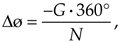
Figure 5-36. FIR filter phase response Hø(m) in degrees: (a) calculated using a 32-point DFT; (b) using a 64-point DFT; (c) using a 128-point DFT.

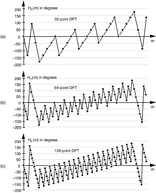
where N is the number of points in the DFT. So, for our S = 25-tap filter in Figure 5-34(a), G = 12, and Dø is equal to –12 · 360°/32 = –135° in Figure 5-36(a), and Dø is –33.75° in Figure 5-36(c). If we look carefully at the sample values in Figure 5-36(a), we'll see that they're all included within the samples in Figures 5-36(b) and 5-36(c).

Let's conclude this FIR phase discussion by reiterating the meaning of phase response. The phase, or phase delay, at the output of an FIR filter is the phase of the first output sample relative to the phase of the filter's first input sample. Over the passband, that phase shift, of course, is a linear function of frequency. This will be true only as long as the filter has symmetrical coefficients. Figure 5-10 is a good illustration of an FIR filter's output phase delay.

For FIR filters, the output phase shift measured in degrees, for the passband frequency f = mfs/N, is expressed as

Equation 5-25

We can illustrate Eq. (5-25) and show the relationship between the phase responses in Figure 5-36, by considering the phase delay associated with the frequency of fs/32 in Table 5-2. The subject of group delay is described further in Appendix F, where an example of envelope delay distortion, due to a filter's nonlinear phase, is illustrated.

Table 5-2. Values Used in Eq. (5-25) for the Frequency fs/32