WINDOWS
Windowing reduces DFT leakage by minimizing the magnitude of Eq. (3-25)'s sinc function's sin(x)/x sidelobes shown in Figure 3-9. We do this by forcing the amplitude of the input time sequence at both the beginning and the end of the sample interval to go smoothly toward a single common amplitude value. Figure 3-15 shows how this process works. If we consider the infinite-duration time signal shown in Figure 3-15(a), a DFT can only be performed over a finite-time sample interval like that shown in Figure 3-15(c). We can think of the DFT input signal in Figure 3-15(c) as the product of an input signal existing for all time, Figure 3-15(a), and the rectangular window whose magnitude is 1 over the sample interval shown in Figure 3-15(b). Anytime we take the DFT of a finite-extent input sequence we are, by default, multiplying that sequence by a window of all ones and effectively multiplying the input values outside that window by zeros. As it turns out, Eq. (3-25)'s sinc function's sin(x)/x shape, shown in Figure 3-9, is caused by this rectangular window because the continuous Fourier transform of the rectangular window in Figure 3-15(b) is the sinc function.
Figure 3-15. Minimizing sample interval endpoint discontinuities: (a) infinite duration input sinusoid; (b) rectangular window due to finite-time sample interval; (c) product of rectangular window and infinite-duration input sinusoid; (d) triangular window function; (e) product of triangular window and infinite-duration input sinusoid; (f) Hanning window function; (g) product of Hanning window and infinite-duration input sinusoid; (h) Hamming window function.
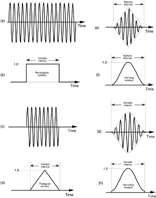
As we'll soon see, it's the rectangular window's abrupt changes between one and zero that are the cause of the sidelobes in the the sin(x)/x sinc function. To minimize the spectral leakage caused by those sidelobes, we have to reduce the sidelobe amplitudes by using window functions other than the rectangular window. Imagine if we multiplied our DFT input, Figure 3-15(c), by the triangular window function shown in Figure 3-15(d) to obtain the windowed input signal shown in Figure 3-15(e). Notice that the values of our final input signal appear to be the same at the beginning and end of the sample interval in Figure 3-15(e). The reduced discontinuity decreases the level of relatively high frequency components in our overall DFT output; that is, our DFT bin sidelobe levels are reduced in magnitude using a triangular window. There are other window functions that reduce leakage even more than the triangular window, such as the Hanning window in Figure 3-15(f). The product of the window in Figure 3-15(f) and the input sequence provides the signal shown in Figure 3-15(g) as the input to the DFT. Another common window function is the Hamming window shown in Figure 3-15(h). It's much like the Hanning window, but it's raised on a pedestal.
Before we see exactly how well these windows minimize DFT leakage, let's define them mathematically. Assuming that our original N input signal samples are indexed by n, where 0  n
n  N–1, we'll call the N time-domain window coefficients w(n); that is, an input sequence x(n) is multiplied by the corresponding window w(n) coefficients before the DFT is performed. So the DFT of the windowed x(n) input sequence, Xw(m), takes the form of

To use window functions, we need mathematical expression of them in terms of n. The following expressions define our window function coefficients:
Rectangular window: (also called the uniform, or boxcar, window)
Equation 3-27

Triangular window: (very similar to the Bartlett[3], and Parzen[4,5] windows)
Equation 3-28
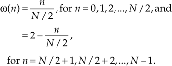
Hanning window: (also called the raised cosine, Hann, or von Hann window)
Equation 3-29

Hamming window:
Equation 3-30

If we plot the w(n) values from Eqs. (3-27) through (3-30), we'd get the corresponding window functions like those in Figures 3-15(b), 3-15(d), 3-15(f), and 3-15(h).[ ]
]
[
] In the literature, the equations for window functions depend on the range of the sample index n. We define n to be in the range 0 < n < N–1. Some authors define n to be in the range –N/2 < n < N/2, in which case, for example, the expression for the Hanning window would have a sign change and be w(n) = 0.5 + 0.5cos(2pn/N–1).
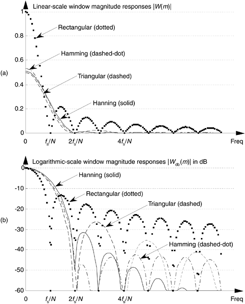
The rectangular window's amplitude response is the yardstick we normally use to evaluate another window function's amplitude response; that is, we typically get an appreciation for a window's response by comparing it to the rectangular window that exhibits the magnitude response shown in Figure 3-9(b). The rectangular window's sin(x)/x magnitude response, |W(m)|, is repeated in Figure 3-16(a). Also included in Figure 3-16(a) are the Hamming, Hanning, and triangular window magnitude responses. (The frequency axis in Figure 3-16 is such that the curves show the response of a single N-point DFT bin when the various window functions are used.) We can see that the last three windows give reduced sidelobe levels relative to the rectangular window. Because the Hamming, Hanning, and triangular windows reduce the time-domain signal levels applied to the DFT, their main lobe peak values are reduced relative to the rectangular window. (Because of the near-zero w(n) coefficients at the beginning and end of the sample interval, this signal level loss is called the processing gain, or loss, of a window.) Be that as it may, we're primarily interested in the windows' sidelobe levels, which are difficult to see in Figure 3-16(a)'s linear scale. We will avoid this difficulty by plotting the windows' magnitude responses on a logarithmic decibel scale, and normalize each plot so its main lobe peak values are zero dB. (Appendix E provides a discussion of the origin and utility of measuring frequency-domain responses on a logarithmic scale using decibels.) Defining the log magnitude response to be |WdB(m)|, we get |WdB(m)| by using the expression
Figure 3-16. Window magnitude responses: (a) |W(m)| on a linear scale; (b) |WdB(m)| on a normalized logarithmic scale.
Equation 3-31

(The |W(0)| term in the denominator of Eq. (3-31) is the value of W(m) at the peak of the main lobe when m = 0.) The |WdB(m)| curves for the various window functions are shown in Figure 3-16(b). Now we can really see how the various window sidelobe responses compare to each other.
Looking at the rectangular window's magnitude response we see that its main lobe is the most narrow, fs/N. However, unfortunately, its first sidelobe level is only –13 dB below the main lobe peak, which is not so good. (Notice that we're only showing the positive frequency portion of the window responses in Figure 3-16.) The triangular window has reduced sidelobe levels, but the price we've paid is that the triangular window's main lobe width is twice as wide as that of the rectangular window's. The various nonrectangular windows' wide main lobes degrade the windowed DFT's frequency resolution by almost a factor of two. However, as we'll see, the important benefits of leakage reduction usually outweigh the loss in DFT frequency resolution.
Notice the further reduction of the first sidelobe level, and the rapid sidelobe roll-off of the Hanning window. The Hamming window has even lower first sidelobe levels, but this window's sidelobes roll off slowly relative to the Hanning window. This means that leakage three or four bins away from the center bin is lower for the Hamming window than for the Hanning window, and leakage a half dozen or so bins away from the center bin is lower for the Hanning window than for the Hamming window.
When we apply the Hanning window to Figure 3-8(a)'s 3.4 cycles per sample interval example, we end up with the DFT input shown in Figure 3-17(a) under the Hanning window envelope. The DFT outputs for the windowed waveform are shown in Figure 3-17(b) along with the DFT results with no windowing, i.e., the rectangular window. As we expected, the shape of the Hanning window's response looks broader and has a lower peak amplitude, but its sidelobe leakage is noticeably reduced from that of the rectangular window.
Figure 3-17. Hanning window: (a) 64-sample product of a Hanning window and a 3.4 cycles per sample interval input sinewave; (b) Hanning DFT output response vs. rectangular window DFT output response.
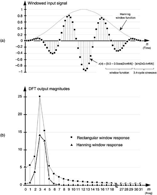
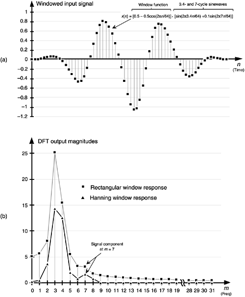
We can demonstrate the benefit of using a window function to help us detect a low-level signal in the presence of a nearby high-level signal. Let's add 64 samples of a 7 cycles per sample interval sinewave, with a peak amplitude of only 0.1, to Figure 3-8(a)'s unity-amplitude 3.4 cycles per sample sinewave. When we apply a Hanning window to the sum of these sinewaves, we get the time-domain input shown in Figure 3-18(a). Had we not windowed the input data, our DFT output would be the squares in Figure 3-18(b) where DFT leakage causes the input signal component at m = 7 to be barely discernible. However, the DFT of the windowed data shown as the triangles in Figure 3-18(b) makes it easier for us to detect the presence of the m = 7 signal component. From a practical standpoint, people who use the DFT to perform real-world signal detection have learned that their overall frequency resolution and signal sensitivity are affected much more by the size and shape of their window function than the mere size of their DFTs.
Figure 3-18. Increased signal detection sensitivity afforded using windowing: (a) 64-sample product of a Hanning window and the sum of a 3.4 cycles and a 7 cycles per sample interval sinewaves; (b) reduced leakage Hanning DFT output response vs. rectangular window DFT output response.
As we become more experienced using window functions on our DFT input data, we'll see how different window functions have their own individual advantages and disadvantages. Furthermore, regardless of the window function used, we've decreased the leakage in our DFT output from that of the rectangular window. There are many different window functions described in the literature of digital signal processing—so many, in fact, that they've been named after just about everyone in the digital signal processing business. It's not that clear that there's a great deal of difference among many of these window functions. What we find is that window selection is a trade-off between main lobe widening, first sidelobe levels, and how fast the sidelobes decrease with increased frequency. The use of any particular window depends on the application[5], and there are many applications.
Windows are used to improve DFT spectrum analysis accuracy[6], to design digital filters[7,8], to simulate antenna radiation patterns, and even in the hardware world to improve the performance of certain mechanical force to voltage conversion devices[9]. So there's plenty of window information available for those readers seeking further knowledge. (The mother of all technical papers on windows is that by Harris[10]. A useful paper by Nuttall corrected and extended some portions of Harris's paper[11].) Again, the best way to appreciate windowing effects is to have access to a computer software package that contains DFT, or FFT, routines and start analyzing windowed signals. (By the way, while we delayed their discussion until Section 5.3, there are two other commonly used window functions that can be used to reduce DFT leakage. They're the Chebyshev and Kaiser window functions, which have adjustable parameters, enabling us to strike a compromise between widening main lobe width and reducing sidelobe levels.)
URL http://proquest.safaribooksonline.com/0131089897/ch03lev1sec9
 |
Amazon |  |
