Section D.3. THE MEAN AND VARIANCE OF RANDOM FUNCTIONS
D 3 THE MEAN AND VARIANCE OF RANDOM FUNCTIONS
To determine the mean or variance of a random function, we use what's called the probability density function. The probability density function (PDF) is a measure of the likelihood of a particular value occurring in some function. We can explain this concept with simple examples of flipping a coin or throwing dice, as illustrated in Figure D-3(a) and (b). The result of flipping a coin can only be one of two possibilities: heads or tails. Figure D-3(a) indicates this PDF and shows that the probability (likelihood) is equal to one-half for both heads and tails. That is, we have an equal chance that the coin side facing up will be heads or tails. The sum of those two probability values is one, meaning that there's a 100% probability that either a head or a tail will occur.
Figure D-3. Simple probability density functions: (a) the probability of flipping a single coin; (b) the probability of a particular sum of the upper faces of two die; (c) the probability of the order of birth of the girl and her sibling.

Figure D-3(b) shows the probability of a particular sum of the upper faces when we throw a pair of dice. This probability function is not uniform because, for example, we're six times more likely to have the die faces add to seven than add to two (snake eyes). We can say that after tossing the dice a large number of times, we should expect that 6/36 = 16.7 percent of those tosses would result in sevens, and 1/36 = 2.8 percent of the time we'll get snake eyes. The sum of those eleven probability values in Figure D-3(b) is also one, telling us that this PDF accounts for all (100%) of the possible outcomes of throwing the dice.
The fact that PDFs must account for all possible results is emphasized in an interesting way in Figure D-3(c). If a woman says, "Of my two children, one is a girl. What's the probability that she has a sister?" Be careful now—curiously enough, the answer to this controversial question is not a 50–50 chance. There are more possibilities to consider than just the girl having a brother or a sister. We can think of all the possible combinations of birth order of two children such that one child is a girl. Because we don't know the gender of the first-born child, there are three gender order possibilities: girl, then boy; boy, then girl; and girl, then girl as shown in Figure D-3(c). So the possibility of the daughter having a sister is 1/3 instead of 1/2! (Believe it.) Again, the sum of those three 1/3rd probability values is one.
Two important features of PDFs are illustrated by the examples in Figure D-3: PDFs are always positive, and the areas under their curves must be equal to unity. The very concept of PDFs make them a positive likelihood that a particular result will occur, and the fact that some result must occur is equivalent to saying that there's a probability of one (100% chance) that we'll have a result. For continuous probability density functions, p( ), we indicate these two characteristics by

and
Equation D-8'

In Section D.1 we illustrated how to calculate the average (mean) and variance of discrete samples. We can also determine these statistical measures for a random function if we know the PDF of the function. Using m to denote the average of a random function of f, then, mf is defined as
Equation D-9

and the variance of f is defined as [3]:
Equation D-10

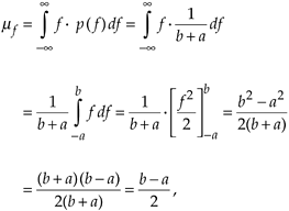
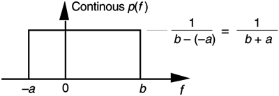
In digital signal processing, we'll encounter continuous probability density functions that are uniform in value similar to the examples in Figure D-3. In these cases, it's easy to use Eqs. (D-9) and (D-10) to determine their average and variance. Figure D-4 illustrates a uniform, continuous PDF indicating a random function whose values have an equal probability of being anywhere in the range from –a to b. From Eq. (D-8), we know that the area under the curve must be unity (i.e., the probability is 100% that the value will be somewhere under the curve). So the amplitude of p(f) must be the area divided by the width, or p(f) = 1/(b + a). From Eq. (D-9), the average of this p(f) is given by
Equation D-11

Figure D-4. Continuous, uniform probability density function.

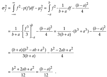
which happens to be the midpoint in the range from –a to b. The variance of the PDF in Figure D-4 is given by
Equation D-12

We use the results of Eqs. (D-11) and (D-12) in Chapter 12 to analyze the errors induced by quantization from analog-to-digital converters and the effects of finite word lengths of hardware registers.
URL http://proquest.safaribooksonline.com/0131089897/app04lev1sec3
 |
Amazon |  |
