DISCRETE SEQUENCES AND THEIR NOTATION
In general, the term signal processing refers to the science of analyzing time-varying physical processes. As such, signal processing is divided into two categories, analog signal processing and digital signal processing. The term analog is used to describe a waveform that's continuous in time and can take on a continuous range of amplitude values. An example of an analog signal is some voltage that can be applied to an oscilloscope, resulting in a continuous display as a function of time. Analog signals can also be applied to a conventional spectrum analyzer to determine their frequency content. The term analog appears to have stemmed from the analog computers used prior to 1980. These computers solved linear differential equations by means of connecting physical (electronic) differentiators and integrators using old-style telephone operator patch cords. That way, a continuous voltage or current in the actual circuit was analogous to some variable in a differential equation, such as speed, temperature, air pressure, etc. (Although the flexibility and speed of modern-day digital computers have since made analog computers obsolete, a good description of the short-lived utility of analog computers can be found in reference [1].) Because present-day signal processing of continuous radio-type signals using resistors, capacitors, operational amplifiers, etc., has nothing to do with analogies, the term analog is actually a misnomer. The more correct term is continuous signal processing for what is today so commonly called analog signal processing. As such, in this book we'll minimize the use of the term analog signals and substitute the phrase continuous signals whenever appropriate.
The term discrete-time signal is used to describe a signal whose independent time variable is quantized so that we know only the value of the signal at discrete instants in time. Thus a discrete-time signal is not represented by a continuous waveform but, instead, a sequence of values. In addition to quantizing time, a discrete-time signal quantizes the signal amplitude. We can illustrate this concept with an example. Think of a continuous sinewave with a peak amplitude of 1 at a frequency fo described by the equation

The frequency fo is measured in hertz (Hz). (In physical systems, we usually measure frequency in units of hertz. One Hz is a single oscillation, or cycle, per second. One kilohertz (kHz) is a thousand Hz, and a megahertz (MHz) is one million Hz.[ ]) With t in Eq. 1-1 representing time in seconds, the fot factor has dimensions of cycles, and the complete 2pfot term is an angle measured in radians.
[
] The dimension for frequency used to be cycles/second; that's why the tuning dials of old radios indicate frequency as kilocycles/second (kcps) or megacycles/second (Mcps). In 1960 the scientific community adopted hertz as the unit of measure for frequency in honor of the German physicist, Heinrich Hertz, who first demonstrated radio wave transmission and reception in 1887.
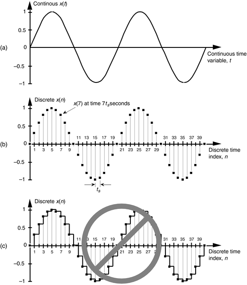
Plotting Eq. (1-1), we get the venerable continuous sinewave curve shown in Figure 1-1(a). If our continuous sinewave represents a physical voltage, we could sample it once every ts seconds using an analog-to-digital converter and represent the sinewave as a sequence of discrete values. Plotting those individual values as dots would give us the discrete waveform in Figure 1-1(b). We say that Figure 1-1(b) is the "discrete-time" version of the continuous signal in Figure 1-1(a). The independent variable t in Eq. (1-1) and Figure 1-1(a) is continuous. The independent index variable n in Figure 1-1(b) is discrete and can have only integer values. That is, index n is used to identify the individual elements of the discrete sequence in Figure 1-1(b).
Figure 1-1. A time-domain sinewave: (a) continuous waveform representation; (b) discrete sample representation; (c) discrete samples with connecting lines.

Do not be tempted to draw lines between the dots in Figure 1-1(b). For some reason, people (particularly those engineers experienced in working with continuous signals) want to connect the dots with straight lines, or the stairstep lines shown in Figure 1-1(c). Don't fall into this innocent-looking trap. Connecting the dots can mislead the beginner into forgetting that the x(n) sequence is nothing more than a list of numbers. Remember, x(n) is a discrete-time sequence of individual values, and each value in that sequence plots as a single dot. It's not that we're ignorant of what lies between the dots of x(n); there is nothing between those dots.
We can reinforce this discrete-time sequence concept by listing those Figure 1-1(b) sampled values as follows:
Equation 1-2

where n represents the time index integer sequence 0, 1, 2, 3, etc., and ts is some constant time period. Those sample values can be represented collectively, and concisely, by the discrete-time expression
Equation 1-3

(Here again, the 2pfonts term is an angle measured in radians.) Notice that the index n in Eq. (1-2) started with a value of 0, instead of 1. There's nothing sacred about this; the first value of n could just as well have been 1, but we start the index n at zero out of habit because doing so allows us to describe the sinewave starting at time zero. The variable x(n) in Eq. (1-3) is read as "the sequence x of n." Equations (1-1) and (1-3) describe what are also referred to as time-domain signals because the independent variables, the continuous time t in Eq. (1-1), and the discrete-time nts values used in Eq. (1-3) are measures of time.
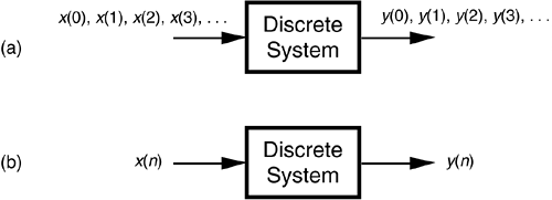
With this notion of a discrete-time signal in mind, let's say that a discrete system is a collection of hardware components, or software routines, that operate on a discrete-time signal sequence. For example, a discrete system could be a process that gives us a discrete output sequence y(0), y(1), y(2), etc., when a discrete input sequence of x(0), x(1), x(2), etc., is applied to the system input as shown in Figure 1-2(a). Again, to keep the notation concise and still keep track of individual elements of the input and output sequences, an abbreviated notation is used as shown in Figure 1-2(b) where n represents the integer sequence 0, 1, 2, 3, etc. Thus, x(n) and y(n) are general variables that represent two separate sequences of numbers. Figure 1-2(b) allows us to describe a system's output with a simple expression such as
Equation 1-4

Figure 1-2. With an input applied, a discrete system provides an output: (a) the input and output are sequences of individual values; (b) input and output using the abbreviated notation of x(n) and y(n).

Illustrating Eq. (1-4), if x(n) is the five-element sequence: x(0) = 1, x(1) = 3, x(2) = 5, x(3) = 7, and x(4) = 9, then y(n) is the five-element sequence y(0) = 1, y(1) = 5, y(2) = 9, y(3) = 13, and y(4) = 17.
The fundamental difference between the way time is represented in continuous and discrete systems leads to a very important difference in how we characterize frequency in continuous and discrete systems. To illustrate, let's reconsider the continuous sinewave in Figure 1-1(a). If it represented a voltage at the end of a cable, we could measure its frequency by applying it to an oscilloscope, a spectrum analyzer, or a frequency counter. We'd have a problem, however, if we were merely given the list of values from Eq. (1-2) and asked to determine the frequency of the waveform they represent. We'd graph those discrete values, and, sure enough, we'd recognize a single sinewave as in Figure 1-1(b). We can say that the sinewave repeats every 20 samples, but there's no way to determine the exact sinewave frequency from the discrete sequence values alone. You can probably see the point we're leading to here. If we knew the time between samples—the sample period ts—we'd be able to determine the absolute frequency of the discrete sinewave. Given that the ts sample period is, say, 0.05 milliseconds/sample, the period of the sinewave is
Equation 1-5

Because the frequency of a sinewave is the reciprocal of its period, we now know that the sinewave's absolute frequency is 1/(1 ms), or 1 kHz. On the other hand, if we found that the sample period was, in fact, 2 milliseconds, the discrete samples in Figure 1-1(b) would represent a sinewave whose period is 40 milliseconds and whose frequency is 25 Hz. The point here is that, in discrete systems, absolute frequency determination in Hz is dependent on the sample frequency fs = 1/ts. We'll be reminded of this dependence throughout the rest of this book.
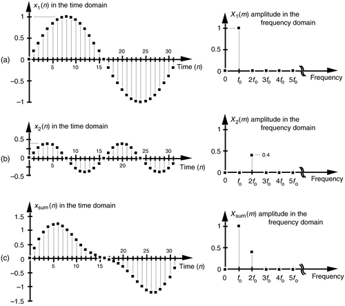
In digital signal processing, we often find it necessary to characterize the frequency content of discrete-time domain signals. When we do so, this frequency representation takes place in what's called the frequency domain. By way of example, let's say we have a discrete sinewave sequence x1(n) with an arbitrary frequency fo Hz as shown on the left side of Figure 1-3(a). We can also describe x1(n) as shown on the right side of Figure 1-3(a) by indicating that it has a frequency of 1, measured in units of fo, and no other frequency content. Although we won't dwell on it just now, notice that the frequency-domain representations in Figure 1-3 are themselves discrete.
Figure 1-3. Time- and frequency-domain graphical representations: (a) sinewave of frequency fo; (b) reduced amplitude sinewave of frequency 2fo; (c) sum of the two sinewaves.

To illustrate our time- and frequency-domain representations further, Figure 1-3(b) shows another discrete sinewave x2(n), whose peak amplitude is 0.4, with a frequency of 2fo. The discrete sample values of x2(n) are expressed by the equation
Equation 1-6

When the two sinewaves, x1(n) and x2(n), are added to produce a new waveform xsum(n), its time-domain equation is
Equation 1-7

and its time- and frequency-domain representations are those given in Figure 1-3(c). We interpret the Xsum(m) frequency-domain depiction, the spectrum, in Figure 1-3(c) to indicate that Xsum(n) has a frequency component of fo Hz and a reduced-amplitude frequency component of 2fo Hz.
Notice three things in Figure 1-3. First, time sequences use lowercase variable names like the "x" in x1(n), and uppercase symbols for frequency-domain variables such as the "X" in X1(m). The term X1(m) is read as "the spectral sequence X sub one of m." Second, because the X1(m) frequency-domain representation of the x1(n) time sequence is itself a sequence (a list of numbers), we use the index "m" to keep track of individual elements in X1(m). We can list frequency-domain sequences just as we did with the time sequence in Eq. (1-2). For example Xsum(m) is listed as

where the frequency index m is the integer sequence 0, 1, 2, 3, etc. Third, because the x1(n) + x2(n) sinewaves have a phase shift of zero degrees relative to each other, we didn't really need to bother depicting this phase relationship in Xsum(m) in Figure 1-3(c). In general, however, phase relationships in frequency-domain sequences are important, and we'll cover that subject in Chapters 3 and 5.
A key point to keep in mind here is that we now know three equivalent ways to describe a discrete-time waveform. Mathematically, we can use a time-domain equation like Eq. (1-6). We can also represent a time-domain waveform graphically as we did on the left side of Figure 1-3, and we can depict its corresponding, discrete, frequency-domain equivalent as that on the right side of Figure 1-3.
As it turns out, the discrete-time domain signals we're concerned with are not only quantized in time; their amplitude values are also quantized. Because we represent all digital quantities with binary numbers, there's a limit to the resolution, or granularity, that we have in representing the values of discrete numbers. Although signal amplitude quantization can be an important consideration—we cover that particular topic in Chapter 12—we won't worry about it just now.
URL http://proquest.safaribooksonline.com/0131089897/ch01lev1sec1
 |
Amazon |  |
