EFFECTS OF FINITE FIXED-POINT BINARY WORD LENGTH
The effects of finite binary word lengths touch all aspects of digital signal processing. Using finite word lengths prevents us from representing values with infinite precision, increases the background noise in our spectral estimation techniques, creates nonideal digital filter responses, induces noise in analog-to-digital (A/D) converter outputs, and can (if we're not careful) lead to wildly inaccurate arithmetic results. The smaller the word lengths, the greater these problems will be. Fortunately, these finite, word-length effects are rather well understood. We can predict their consequences and take steps to minimize any unpleasant surprises. The first finite, word-length effect we'll cover is the errors that occur during the A/D conversion process.
12.3.1 A/D Converter Quantization Errors
Practical A/D converters are constrained to have binary output words of finite length. Commercial A/D converters are categorized by their output word lengths, which are normally in the range from 8 to 16 bits. A typical A/D converter input analog voltage range is from –1 to +1 volt. If we used such an A/D converter having eight-bit output words, the least significant bit would represent
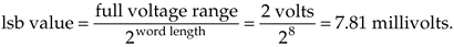
What this means is that we can represent continuous (analog) voltages perfectly as long as they're integral multiples of 7.81 millivolts—any intermediate input voltage will cause the A/D converter to output a best estimate digital data value. The inaccuracies in this process are called quantization errors because an A/D output least significant bit is an indivisible quantity. We illustrate this situation in Figure 12-1(a), where the continuous waveform is being digitized by an eight-bit A/D converter whose output is in the sign-magnitude format. When we start sampling at time t = 0, the continuous waveform happens to have a value of 31.25 millivolts (mv), and our A/D output data word will be exactly correct for sample x(0). At time T when we get the second A/D output word for sample x(1), the continuous voltage is between 0 and –7.81 mv. In this case, the A/D converter outputs a sample value of 10000001 representing –7.81 mv, even though the continuous input was not quite as negative as –7.81mv. The 10000001 A/D output word contains some quantization error. Each successive sample contains quantization error because the A/D's digitized output values must lie on a horizontal dashed line in Figure 12-1(a). The difference between the actual continuous input voltage and the A/D converter's representation of the input is shown as the quantization error in Figure 12-1(b). For an ideal A/D converter, the quantization error, a kind of roundoff noise, can never be greater than ±1/2 an lsb, or ±3.905 mv.
Figure 12-1. Quantization errors: (a) digitized x(n) values of a continuous signal; (b) quantization error between the actual analog signal values and the digitized signal values.
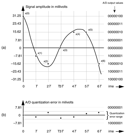
While Figure 12-1(b) shows A/D quantization noise in the time domain, we can also illustrate this noise in the frequency domain. Figure 12-2(a) depicts a continuous sinewave of one cycle over the sample interval shown as the dotted line and a quantized version of the time-domain samples of that wave as the dots. Notice how the quantized version of the wave is constrained to have only integral values, giving it a stair step effect oscillating above and below the true unquantized sinewave. The quantization here is 4 bits, meaning that we have a sign bit and three bits to represent the magnitude of the wave. With three bits, the maximum peak values for the wave are ±7. Figure 12-2(b) shows the discrete Fourier transform (DFT) of a discrete version of the sinewave whose time-domain sample values are not forced to be integers, but have high precision. Notice in this case that the DFT has a nonzero value only at m = 1. On the other hand, Figure 12-2(c) shows the spectrum of the 4-bit quantized samples in Figure 12-2(a), where quantization effects have induced noise components across the entire spectral band. If the quantization noise depictions in Figures 12-1(b) and 12-2(c) look random, that's because they are. As it turns out, even though A/D quantization noise is random, we can still quantify its effects in a useful way.
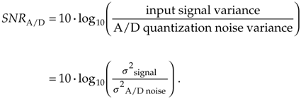
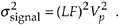
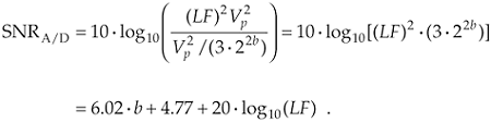
In the field of communications, people often use the notion of output signal-to-noise ratio, or SNR = (signal power)/(noise power), to judge the usefulness of a process or device. We can do likewise and obtain an important expression for the output SNR of an ideal A/D converter, SNRA/D, accounting for finite word-length quantization effects. Because quantization noise is random, we can't explicitly represent its power level, but we can use its statistical equivalent of variance to define SNRA/D measured in decibels as
Figure 12-2. Quantization noise effects: (a) input sinewave applied to a 64-point DFT; (b) theoretical DFT magnitude of high-precision sinewave samples; (c) DFT magnitude of a sinewave quantized to 4 bits.
Equation 12-8
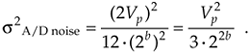
Next, we'll determine an A/D converter's quantization noise variance relative to the converter's maximum input peak voltage Vp. If the full scale (–Vp to +Vp volts) continuous input range of a b-bit A/D converter is 2Vp, a single quantization level q is that voltage range divided by the number of possible A/D output binary values, or q = 2Vp/2b. (In Figure 12-1, for example, the quantization level q is the lsb value of 7.81 mv.) A depiction of the likelihood of encountering any given quantization error value, called the probability density function p(e) of the quantization error, is shown in Figure 12-3.
Figure 12-3. Probability density function of A/D conversion roundoff error (noise).
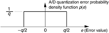
This simple rectangular function has much to tell us. It indicates that there's an equal chance that any error value between –q/2 and +q/2 can occur. By definition, because probability density functions have an area of unity (i.e., the probability is 100 percent that the error will be somewhere under the curve), the amplitude of the p(e) density function must be the area divided by the width, or p(e) = 1/q. From Figure D-4 and Eq. (D-12) in Appendix D, the variance of our uniform p(e) is
Equation 12-9
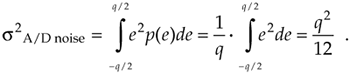
We can now express the A/D noise error variance in terms of A/D parameters by replacing q in Eq. (12-9) with q = 2Vp/2b to get
Equation 12-10
OK, we're halfway to our goal—with Eq. (12-10) giving us the denominator of Eq. (12-8), we need the numerator. To arrive at a general result, let's express the input signal in terms of its root mean square (rms), the A/D converter's peak voltage, and a loading factor LF defined as
Equation 12-11
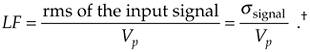
With the loading factor defined as the input rms voltage over the A/D converter's peak input voltage, we square and rearrange Eq. (12-11) to show the signal variance  as
as
Equation 12-12
Substituting Eqs. (12-10) and (12-12) in Eq. (12-8),
Equation 12-13
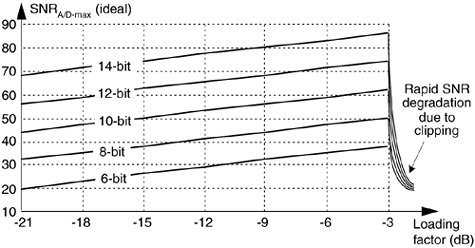
Eq. (12-13) gives us the SNRA/D of an ideal b-bit A/D converter in terms of the loading factor and the number of bits b. Figure 12-4 plots Eq. (12-13) for various A/D word lengths as a function of the loading factor. Notice that the loading factor in Figure 12-4 is never greater than –3dB, because the maximum continuous A/D input peak value must not be greater than Vp volts. Thus, for a sinusoid input, its rms value must not be greater than  volts (3 dB below Vp).
Figure 12-4. SNRA/D of ideal A/D converters as a function of loading factor in dB.
 Recall from Appendix D, Section D.2 that, although the variance s2 is associated with the power of a signal, the standard deviation is associated with the rms value of a signal.
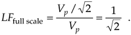
When the input sinewave's peak amplitude is equal to the A/D converter's full-scale voltage Vp, the full-scale LF is
Equation 12-14
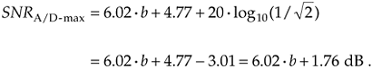
Under this condition, the maximum A/D output SNR from Eq. (12-13) is
Equation 12-15
This discussion of SNR relative to A/D converters means three important things to us:
- An ideal A/D converter will have an SNRA/D defined by Eq. (12-13), so any continuous signal we're trying to digitize with a b-bit A/D converter will never have an SNRA/D greater than Eq. (12-13) after A/D conversion. For example, let's say we want to digitize a continuous signal whose SNR is 55 dB. Using an ideal eight-bit A/D converter with its full-scale SNRA/D of 6.02 · 8 + 1.76 = 49.9 dB from Eq. (12-15), the quantization noise will contaminate the digitized values, and the resultant digital signal's SNR can be no better than 49.9 dB. We'll have lost signal SNR through the A/D conversion process. (A ten-bit A/D, with its ideal SNRA/D
 62 dB, could be used to digitize a 55 dB SNR continuous signal to reduce the SNR degradation caused by quantization noise.) Equations (12-13) and (12-15) apply to ideal A/D converters and don't take into account such additional A/D noise sources as aperture jitter error, missing output bit patterns, and other nonlinearities. So actual A/D converters are likely to have SNRs that are lower than that indicated by theoretical Eq. (12-13). To be safe in practice, it's sensible to assume that SNRA/D-max is 3 to 6 dB lower than indicated by Eq. (12-15).
 - Equation (12-15) is often expressed in the literature, but it can be a little misleading because it's imprudent to force an A/D converter's input to full scale. It's wise to drive an A/D converter to some level below full scale because inadvertent overdriving will lead to signal clipping and will induce distortion in the A/D's output. So Eq. (12-15) is overly optimistic, and, in practice, A/D converter SNRs will be less than indicated by Eq. (12-15). The best approximation for an A/D's SNR is to determine the input signal's rms value that will never (or rarely) overdrive the converter input, and plug that value into Eq. (12-11) to get the loading factor value for use in Eq. (12-13).[] Again, using an A/D converter with a wider word length will alleviate this problem by increasing the available SNRA/D.
[
] By the way, some folks use the term crest factor to describe how hard an A/D converter's input is being driven. The crest factor is the reciprocal of the loading factor, or CF = Vp/(rms of the input signal). - Remember now, real-world continuous signals always have their own inherent continuous SNR, so using an A/D converter whose SNRA/D is a great deal larger than the continuous signal's SNR serves no purpose. In this case, we'd be using the A/D converter's extra bits to digitize the continuous signal's noise to a greater degree of accuracy.
A word of caution is appropriate here concerning our analysis of A/D converter quantization errors. The derivations of Eqs. (12-13) and (12-15) are based upon three assumptions:
- The cause of A/D quantization errors is a stationary random process; that is, the performance of the A/D converter does not change over time. Given the same continuous input voltage, we always expect an A/D converter to provide exactly the same output binary code.
- The probability density function of the A/D quantization error is uniform. We're assuming that the A/D converter is ideal in its operation and all possible errors between –q/2 and +q/2 are equally likely. An A/D converter having stuck bits or missing output codes would violate this assumption. High-quality A/D converters being driven by continuous signals that cross many quantization levels will result in our desired uniform quantization noise probability density function.
- The A/D quantization errors are uncorrelated with the continuous input signal. If we were to digitize a single continuous sinewave whose frequency was harmonically related to the A/D sample rate, we'd end up sampling the same input voltage repeatedly and the quantization error sequence would not be random. The quantization error would be predictable and repetitive, and our quantization noise variance derivation would be invalid. In practice, complicated continuous signals such as music or speech, with their rich spectral content, avoid this problem.
To conclude our discussion of A/D converters, let's consider one last topic. In the literature the reader is likely to encounter the expression
Equation 12-16
Equation (12-16) is used by test equipment manufacturers to specify the sensitivity of test instruments using a beff parameter known as the number of effective bits, or effective number of bits (ENOB) [3–8]. Equation (12-16) is merely Eq. (12-15) solved for b. Test equipment manufacturers measure the actual SNR of their product indicating its ability to capture continuous input signals relative to the instrument's inherent noise characteristics. Given this true SNR, they use Eq. (12-16) to determine the beff value for advertisement in their product literature. The larger beff, the greater the continuous voltage that can be accurately digitized relative to the equipment's intrinsic quantization noise.
12.3.2 Data Overflow
The next finite, word-length effect we'll consider is called overflow. Overflow is what happens when the result of an arithmetic operation has too many bits, or digits, to be represented in the hardware registers designed to contain that result. We can demonstrate this situation to ourselves rather easily using a simple four-function, eight-digit pocket calculator. The sum of a decimal 9.9999999 plus 1.0 is 10.9999999, but on an eight-digit calculator the sum is 10.999999 as
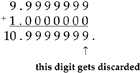
The hardware registers, which contain the arithmetic result and drive the calculator's display, can hold only eight decimal digits; so the least significant digit is discarded (of course). Although the above error is less than one part in ten million, overflow effects can be striking when we work with large numbers. If we use our calculator to add 99,999,999 plus 1, instead of getting the correct result of 100 million, we'll get a result of 1. Now that's an authentic overflow error!
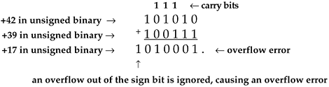
Let's illustrate overflow effects with examples more closely related to our discussion of binary number formats. First, adding two unsigned binary numbers is as straightforward as adding two decimal numbers. The sum of 42 plus 39 is 81, or
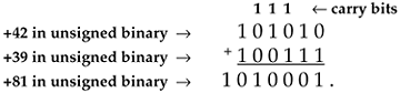
In this case, two 6-bit binary numbers required 7 bits to represent the results. The general rule is the sum of m individual b-bit binary numbers can require as many as [b + log2(m)] bits to represent the results. So, for example, a 24-bit result register (accumulator) is needed to accumulate the sum of sixteen 20-bit binary numbers, or 20 + log2(16) = 24. The sum of 256 eight-bit words requires an accumulator whose word length is [8 + log2(256)], or 16 bits, to ensure that no overflow errors occur.
In the preceding example, if our accumulator word length was 6 bits, an overflow error occurs as
Here, the most significant bit of the result overflowed the 6-bit accumulator, and an error occurred.
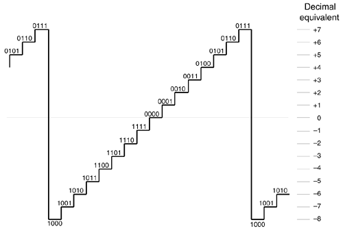
With regard to overflow errors, the two's complement binary format has two interesting characteristics. First, under certain conditions, overflow during the summation of two numbers causes no error. Second, with multiple summations, intermediate overflow errors cause no problems if the final magnitude of the sum of the b-bit two's complement numbers is less than 2b–1. Let's illustrate these properties by considering the four-bit two's complement format in Figure 12-5, whose binary values are taken from Table 12-2.
Figure 12-5. Four-bit two's complement binary numbers.
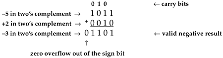
The first property of two's complement overflow, which sometimes causes no errors, can be shown by the following examples:
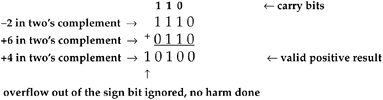
Then again, the following examples show how two's complement overflow sometimes does cause errors:
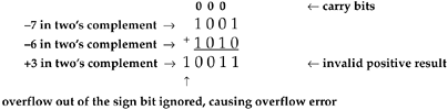
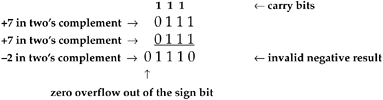
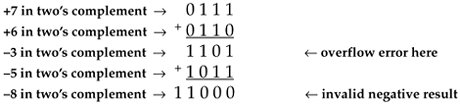
The rule with two's complement addition is if the carry bit into the sign bit is the same as the overflow bit out of the sign bit, the overflow bit can be ignored, causing no errors; if the carry bit into the sign bit is different from the overflow bit out of the sign bit, the result is invalid. An even more interesting property of two's complement numbers is that a series of b-bit word summations can be performed where intermediate sums are invalid, but the final sum will be correct if its magnitude is less than 2b–1. We show this by the following example. If we add a +6 to a +7, and then add a –7, we'll encounter an intermediate overflow error but our final sum will be correct as
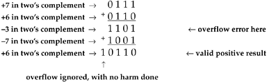
The magnitude of the sum of the three four-bit numbers was less than 24–1 (<8), so our result was valid. If we add a +6 to a +7, and next add a –5, we'll encounter an intermediate overflow error, and our final sum will also be in error because its magnitude is not less than 8.
Another situation where overflow problems are conspicuous is during the calculation of the fast Fourier transform (FFT). It's difficult at first to imagine that multiplying complex numbers by sines and cosines can lead to excessive data word growth—particularly because sines and cosines are never greater than unity. Well, we can show how FFT data word growth occurs by considering a decimation-in-time FFT butterfly from Figure 4-14(c) repeated here as Figure 12-6, and grinding through a little algebra. The expression for the x' output of this FFT butterfly, from Eq. (4-26), is
Equation 12-17

Figure 12-6. Single decimation-in-time FFT butterfly.
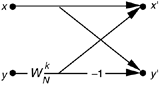
Breaking up the butterfly's x and y inputs into their real and imaginary parts and remembering that  , we can express Eq. (12-17) as
Equation 12-18

If we let a be the twiddle factor angle of 2pk/N, and recall that e–ja = cos(a) – jsin(a), we can simplify Eq. (12-18) as
Equation 12-19
If we look, for example, at just the real part of the x' output, x'real, it comprises the three terms
Equation 12-20

If xreal, yreal, and yimag are of unity value when they enter the butterfly and the twiddle factor angle a = 2pk/N happens to be p/4 = 45o, then, x'real can be greater than 2 as
Equation 12-21
So we see that the real part of a complex number can more than double in magnitude in a single stage of an FFT. The imaginary part of a complex number is equally likely to more than double in magnitude in a single FFT stage. Without mitigating this word growth problem, overflow errors could render an FFT algorithm useless.
OK, overflow problems are handled in one of two ways—by truncation or rounding—each inducing its own individual kind of quantization errors, as we shall see.
12.3.3 Truncation
Truncation is the process where a data value is represented by the largest quantization level that is less than or equal to that data value. If we're quantizing to integral values, for example, the real value 1.2 would be quantized to 1. An example of truncation to integral values is shown in Figure 12-7(a), where all values of x in the range of 0  x < 1 are set equal to 0, values of x in the range of 1 x < 2 are set equal to 1, x values in the range of 2 x < 3 are set equal to 2, and so on.
Figure 12-7. Truncation: (a) quantization nonlinearities; (b) error probability density function.
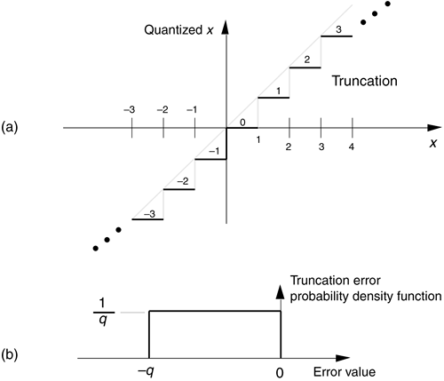
As we did with A/D converter quantization errors, we can call upon the concept of probability density functions to characterize the errors induced by truncation. The probability density function of truncation errors, in terms of the quantization level, is shown in Figure 12-7(b). In Figure 12-7(a) the quantization level q is 1, so, in this case, we can have truncation errors as great as –1. Drawing upon our results from Eqs. (D-11) and (D-12) in Appendix D, the mean and variance of our uniform truncation probability density function are expressed as
Equation 12-22
and
Equation 12-23
In a sense, truncation error is the price we pay for the privilege of using integer binary arithmetic. One aspect of this is the error introduced when we use truncation to implement division by some integral power of 2. We often speak of a quick way of dividing a binary value by 2T is to shift that binary word T bits to the right; that is, we're truncating the data value (not the data word) by lopping off the rightmost T bits after the shift. For example, let's say we have the value 31 represented by the five-bit binary number 111112, and we want to divide it by 16 through shifting the bits T = 4 places to the right and ignoring (truncating) those shifted bits. After the right shift and truncation, we'd have a binary quotient of 31/16 = 000012. Well, we see the significance of the problem because our quick division gave us an answer of one instead of the correct 31/16 = 1.9375. Our division-by-truncation error here is almost 50 percent of the correct answer. Had our original dividend been a 63 represented by the six-bit binary number 1111112, dividing it by 16 through a four-bit shift would give us an answer of binary 0000112, or decimal three. The correct answer, of course, is 63/16 = 3.9375. In this case the percentage error is 0.9375/3.9375, or about 23.8 percent. So, the larger the dividend, the lower the truncation error.
If we study these kinds of errors, we'll find that the resulting truncation error depends on three things: the number of value bits shifted and truncated, the values of the truncated bits (were those dropped bits ones or zeros), and the magnitude of the binary number left over after truncation. Although a complete analysis of these truncation errors is beyond the scope of this book, we can quantify the maximum error that can occur with our division-by-truncation scheme when using binary integer arithmetic. The worst case scenario is when all of the T bits to be truncated are ones. For binary integral numbers the value of T bits, all ones, to the right of the binary point is 1 – 2–T. If the resulting quotient N is small, the significance of those truncated ones aggravates the error. We can normalize the maximum division error by comparing it to the correct quotient using a percentage. So the maximum percentage error of the binary quotient N after truncation for a T-bit right shift, when the truncated bits are all ones, is
Equation 12-24
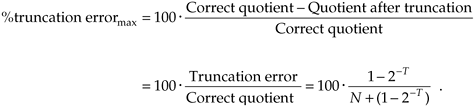
Let's plug a few numbers into Eq. (12-24) to understand its significance. In the first example above, 31/16, where T = 4 and the resulting binary quotient was N = 1, the percentage error is

Plotting Eq. (12-24) for three different shift values as functions of the quotient, N, after truncation results in Figure 12-8.
Figure 12-8. Maximum error when data shifting and truncation are used to implement division by 2T. T = 1 is division by 2; T = 2 is division by 4; and T = 8 is division by 256.
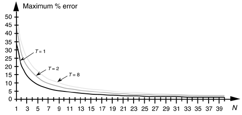
So, to minimize this type of division error, we need to keep the resulting binary quotient N, after the division, as large as possible. Remember, Eq. (12-24) was a worst case condition where all of the truncated bits were ones. On the other hand, if all of the truncated bits happened to be zeros, the error will be zero. In practice, the errors will be somewhere between these two extremes. A practical example of how division-by-truncation can cause serious numerical errors is given in Reference [9].
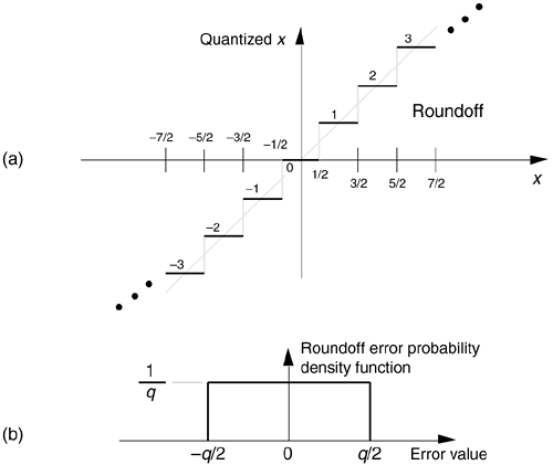
12.3.4 Data Rounding
Rounding is an alternate process of dealing with overflow errors where a data value is represented by, or rounded off to, its nearest quantization level. If we're quantizing to integral values, the number 1.2 would be quantized to 1, and the number 1.6 would be quantized to 2. This is shown in Figure 12-9(a), where all values of x in the range of –0.5 x < 0.5 are set equal to 0, values of x in the range of 0.5 x < 1.5 are set equal to 1, x values in the range of 1.5 x < 2.5 are set equal to 2, etc. The probability density function of the error induced by rounding, in terms of the quantization level, is shown in Figure 12-9(b). In Figure 12-9(a), the quantization level q is 1, so, in this case, we can have truncation error magnitudes no greater than q/2, or 1/2. Again, using our Eqs. (D-11) and (D-12) results from Appendix D, the mean and variance of our uniform roundoff probability density function are expressed as
Figure 12-9. Roundoff: (a) quantization nonlinearities; (b) error probability density function.
Equation 12-25
and
Equation 12-26
Because the mean (average) and maximum error possibly induced by roundoff is less than that of truncation, rounding is generally preferred, in practice, to minimize overflow errors.
In digital signal processing, statistical analysis of quantization error effects is exceedingly complicated. Analytical results depend on the types of quantization errors, the magnitude of the data being represented, the numerical format used, and which of the many FFT or digital filter structures we happen to use. Be that as it may, digital signal processing experts have developed simplified error models whose analysis has proved useful. Although discussion of these analysis techniques and their results is beyond the scope of this introductory text, many references are available for the energetic reader[10–18]. (Reference [11] has an extensive reference list of its own on the topic of quantization error analysis.)
Again, the overflow problems using fixed-point binary formats—that we try to alleviate with truncation or roundoff—arise because so many digital signal processing algorithms comprise large numbers of additions or multiplications. This obstacle, particularly in hardware implementations of digital filters and the FFT, is avoided by hardware designers through the use of floating-point binary formats.
URL http://proquest.safaribooksonline.com/0131089897/ch12lev1sec3
| Amazon | ||
