CONVOLUTION IN FIR FILTERS
OK, here's where we get serious about understanding the mathematics behind FIR filters. We can graphically depict Eq. (5-3)'s and Figure 5-4's calculations as shown in Figure 5-5. Also, let's be formal and use the standard notation of digital filters for indexing the input samples and the filter coefficients by starting with an initial index value of zero; that is, we'll call the initial input value the 0th sample x(0). The next input sample is represented by the term x(1), the following input sample is called x(2), and so on. Likewise, our five coefficient values will be indexed from zero to four, h(0) through h(4). (This indexing scheme makes the equations describing our example consistent with conventional filter notation found in the literature.)
Figure 5-5. Averaging filter convolution: (a) first five input samples aligned with the stationary filter coefficients, index n = 4; (b) input samples shift to the right and index n = 5; (c) index n = 6; (d) index n = 7; (e) index n = 8.
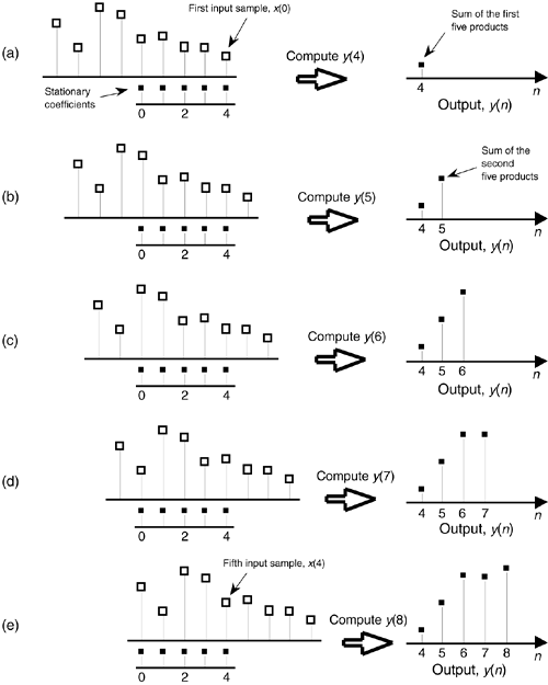
In Eq. (5-3) we used the factor of 1/5 as the filter coefficients multiplied by our averaging filter's input samples. The left side of Figure 5-5 shows the alignment of those coefficients, black squares, with the filter input sample values represented by the white squares. Notice in Figure 5-5(a) through 5-5(e) that we're marching the input samples to the right, and, at each step, we calculate the filter output sample value using Eq. (5-3). The output samples on the right side of Figure 5-5 match the first five values represented by the black squares in Figure 5-2. The input samples in Figure 5-5 are those values represented by the white squares in Figure 5-2. Notice that the time order of the inputs in Figure 5-5 has been reversed from the input sequence order in Figure 5-2! That is, the input sequence has been flipped in the time-domain in Figure 5-5. This time order reversal is what happens to the input data using the filter structure in Figure 5-4.
Repeating the first part of Eq. (5-3) and omitting the subscript on the output term, our original FIR filter's y(n)th output is given by

Because we'll explore filters whose coefficients are not all the same value, we need to represent the individual filter coefficients by a variable, such as the term h(k), for example. Thus we can rewrite the averaging filter's output from Eq. (5-4) in a more general way as
Equation 5-5

where h(0) through h(4) all equal 1/5. Equation (5-5) is a concise way of describing the filter structure in Figure 5-4 and the process illustrated in Figure 5-5.
Let's take Eq. (5-5) one step further and say, for a general M-tap FIR filter, the nth output is
Equation 5-6

Well, there it is. Eq. (5-6) is the infamous convolution equation as it applies to digital FIR filters. Beginners in the field of digital signal processing often have trouble understanding the concept of convolution. It need not be that way. Eq. (5-6) is merely a series of multiplications followed by the addition of the products. The process is actually rather simple. We just flip the time order of an input sample sequence and start stepping the flipped sequence across the filter's coefficients as shown in Figure 5-5. For each new filter input sample, we sum a series of products to compute a single filter output value.
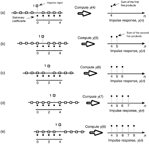
Let's pause for a moment and introduce a new term that's important to keep in mind, the impulse response. The impulse response of a filter is exactly what its name implies—it's the filter's output time-domain sequence when the input is a single unity-valued sample (impulse) preceded and followed by zero-valued samples. Figure 5-6 illustrates this idea in the same way we determined the filter's output sequence in Figure 5-5. The left side of Figure 5-6 shows the alignment of the filter coefficients, black squares, with the filter input impulse sample values represented by the white squares. Again, in Figure 5-6(a) through 5-6(e) we're shifting the input samples to the right, and, at each step, we calculate the filter output sample value using Eq. (5-4). The output samples on the right side of Figure 5-6 are the filter's impulse response. Notice the key point here: the FIR filter's impulse response is identical to the five filter coefficient values. For this reason, the terms FIR filter coefficients and impulse response are synonymous. Thus, when someone refers to the impulse response of an FIR filter, they're also talking about the coefficients.
Figure 5-6. Convolution of filter coefficients and an input impulse to obtain the filter's output impulse response: (a) impulse sample aligned with the first filter coefficient, index n = 4; (b) impulse sample shifts to the right and index n = 5; (c) index n = 6; (d) index n = 7; (e) index n = 8.
Returning to our averaging filter, recall that coefficients (or impulse response) h(0) through h(4) were all equal to 1/5. As it turns out, our filter's performance can be improved by using coefficients whose values are not all the same. By performance we mean how well the filter passes desired signals and attenuates unwanted signals. We judge that performance by determining the shape of the filter's frequency-domain response that we obtain by the convolution property of linear systems. To describe this concept, let's repeat Eq. (5-6) using the abbreviated notation of
Equation 5-7

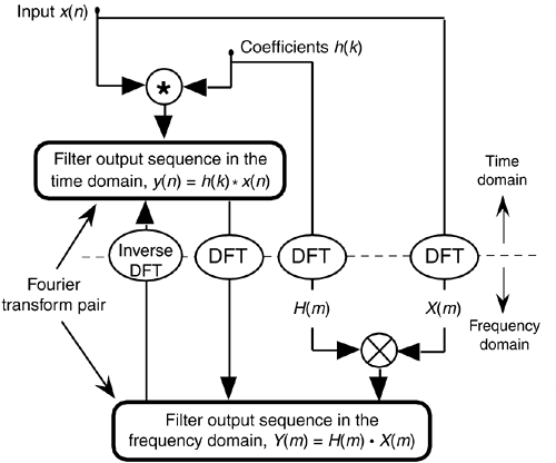
where the * symbol means convolution. (Equation 5-7 is read as "y of n equals the convolution of h of k and x of n.") The process of convolution, as it applies to FIR filters is as follows: the discrete Fourier transform (DFT) of the convolution of a filter's impulse response (coefficients) and an input sequence is equal to the product of the spectrum of the input sequence and the DFT of the impulse response. The idea we're trying to convey here is that if two time-domain sequences h(k) and x(n) have DFTs of H(m) and X(m), respectively, then the DFT of y(n) = h(k) * x(n) is H(m) · X(m). Making this point in a more compact way, we state this relationship with the expression
Equation 5-8

With IDFT indicating the inverse DFT, Eq. (5-8) indicates that two sequences resulting from h(k)*x(n) and H(m)·X(m) are Fourier transform pairs. So taking the DFT of h(k)*x(n) gives us the product H(m)·X(m) that is the spectrum of our filter output Y(m). Likewise, we can determine h(k)*x(n) by taking the inverse DFT of H(m) · X(m). The very important conclusion to learn from Eq. (5-8) is that convolution in the time domain is equivalent to multiplication in the frequency domain. To help us appreciate this principle, Figure 5-7 sketches the relationship between convolution in the time domain and multiplication in the frequency domain. The process of convolution with regard to linear systems is discussed in more detail in Section 5.9. The beginner is encouraged to review that material to get a general idea of why and when the convolution process can be used to analyze digital filters.
Figure 5-7. Relationships of convolution as applied to FIR digital filters.
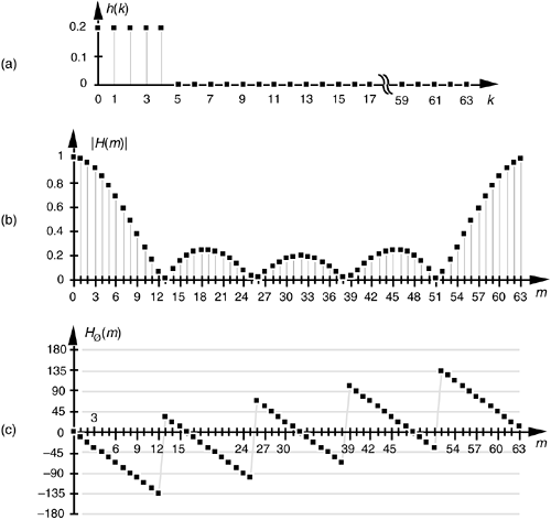
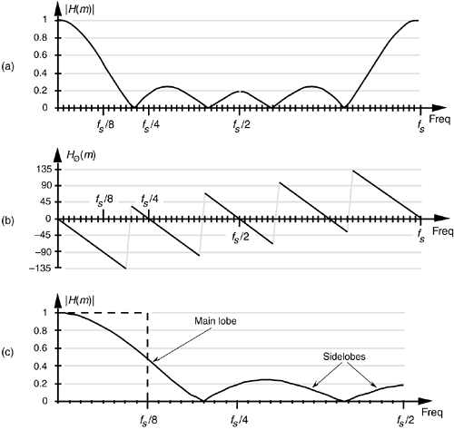
Equation (5-8) and the relationships in Figure 5-7 tell us what we need to do to determine the frequency response of an FIR filter. The product X(m) · H(m) is the DFT of the filter output. Because X(m) is the DFT of the filter's input sequence, the frequency response of the filter is then defined as H(m), the DFT of filter's impulse response h(k).[] Getting back to our original problem, we can determine our averaging filter's frequency-domain response by taking the DFT of the individual filter coefficients (impulse response) in Eq. (5-4). If we take the five h(k) coefficient values of 1/5 and append 59 zeros, we have the sequence depicted in Figure 5-8(a). Performing a 64-point DFT on that sequence, and normalizing the DFT magnitudes, gives us the filter's frequency magnitude response |H(m)| in Figure 5-8(b) and phase response shown in Figure 5-8(c).[
 ] H(m) is our old friend, the sin(x)/x function from Section 3.13.
[] We use the term impulse response here, instead of coefficients, because this concept also applies to IIR filters. IIR filter frequency responses are also equal to the DFT of their impulse responses.
[
] There's nothing sacred about using a 64-point DFT here. We could just as well have appended only enough zeros to take a 16- or 32-point FFT. We chose 64 points to get a frequency resolution that would make the shape of the response in Figure 5-8(b) reasonably smooth. Remember, the more points in the FFT, the finer the frequency resolution—right?
Figure 5-8. Averaging FIR filter: (a) filter coefficient sequence h(k) with appended zeros; (b) normalized discrete frequency magnitude response |H(m)| of the h(k) filter coefficients; (c) phase-angle response of H(m) in degrees.
Let's relate the discrete frequency response samples in Figures 5-8(b) and 5-8(c) to the physical dimension of the sample frequency fs. We know, from Section 3.5 and our experience with the DFT, that the m = N/2 discrete frequency sample, m = 32 in this case, is equal to the folding frequency, or half the sample rate, fs/2. Keeping this in mind, we can convert the discrete frequency axis in Figure 5-8 to that shown in Figure 5-9. In Figure 5-9(a), notice that the filter's magnitude response is, of course, periodic in the frequency domain with a period of the equivalent sample rate fs. Because we're primarily interested in the filter's response between 0 and half the sample rate, Figure 5-9(c) shows that frequency band in greater detail affirming the notion that averaging behaves like a low-pass filter. It's a relatively poor low-pass filter compared to an arbitrary, ideal low-pass filter indicated by the dashed lines in Figure 5-9(c), but our averaging filter will attenuate higher frequency inputs relative to its response to low-frequency input signals.
Figure 5-9. Averaging FIR filter frequency response shown as continuous curves: (a) normalized frequency magnitude response, |H(m)|; (b) phase angle response of H(m) in degrees; (c) the filter's magnitude response between zero Hz and half the sample rate, fs/2 Hz.
We can demonstrate this by way of example. Suppose we applied a low-frequency sinew ave to the averaging FIR filter, as shown by the white squares in Figure 5-10(a), and that the input sinewave's frequency is fs/32 and its peak amplitude is unity. The filter output in this case would be a sinewave of frequency fs/32, but its peak amplitude would be reduced to a value of 0.96, and the output sinewave is delayed by a phase angle of 22.5°. Next, if we applied a higher frequency sinewave of 3fs/32 to the FIR filter as shown in Figure 5-10(b), the filter output would, then, be a sinewave of frequency 3fs/32, but its peak amplitude is even further reduced to a value of 0.69. In addition, the Figure 5-10(b) output sinewave has an even larger phase angle delay of 67.5°. Although the output amplitudes and phase delays in Figure 5-10 were measured values from actually performing a 5-tap FIR filter process on the input sinewave samples, we could have obtained those amplitude and phase delay values directly from Figures 5-8(a) and 5-8(b). The emphasis here is that we don't have to implement an FIR filter and apply various sinewave inputs to discover what its frequency response will be. We need merely take the DFT of the FIR filter's coefficients (impulse response) to determine the filter's frequency response as we did for Figure 5-8.
Figure 5-10. Averaging FIR filter input and output responses: (a) with an input sinewave of frequency fs/32; (b) with an input sinewave of frequency 3fs/32.
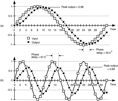
Figure 5-11 is another depiction of how well our 5-tap averaging FIR filter performs, where the dashed line is the filter's magnitude response |H(m)|, and the shaded line is the |X(m)| magnitude spectrum of the filter's input values (the white squares in Figure 5-2). The solid line is the magnitude spectrum of the filter's output sequence, which is shown by the black squares in Figure 5-2. So in Figure 5-11, the solid output spectrum is the product of the dashed filter response curve and the shaded input spectrum, or |X(m)·H(m)|. Again, we see that our averager does indeed attenuate the higher frequency portion of the input spectrum.
Figure 5-11. Averaging FIR filter input magnitude spectrum, frequency magnitude response, and output magnitude spectrum.

Let's pause for a moment to let all of this soak in a little. So far we've gone through the averaging filter example to establish that
- FIR filters perform time-domain convolution by summing the products of the shifted input samples and a sequence of filter coefficients,
- an FIR filter's output sequence is equal to the convolution of the input sequence and a filter's impulse response (coefficients),
- an FIR filter's frequency response is the DFT of the filter's impulse response,
- an FIR filter's output spectrum is the product of the input spectrum and the filter's frequency response, and
- convolution in the time domain and multiplication in the frequency domain are Fourier transform pairs.
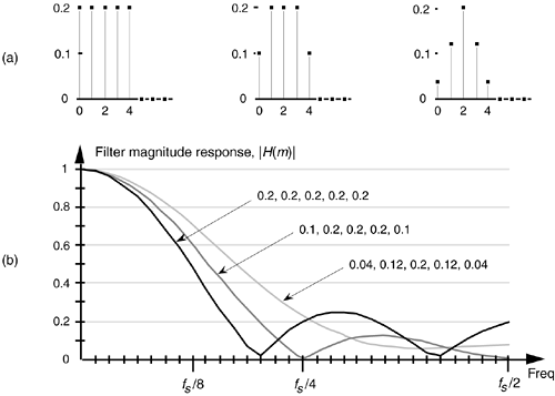
OK, here's where FIR filters start to get really interesting. Let's change the values of the five filter coefficients to modify the frequency response of our 5-tap, low-pass filter. In fact, Figure 5-12(a) shows our original five filter coefficients and two other arbitrary sets of 5-tap coefficients. Figure 5-12(b) compares the frequency magnitude responses of those three sets of coefficients. Again, the frequency responses are obtained by taking the DFT of the three individual sets of coefficients and plotting the magnitude of the transforms, as we did for Figure 5-9(c). So we see three important characteristics in Figure 5-12. First, as we expected, different sets of coefficients give us different frequency magnitude responses. Second, a sudden change in the values of the coefficient sequence, such as the 0.2 to 0 transition in the first coefficient set, causes ripples, or sidelobes, in the frequency response. Third, if we minimize the suddenness of the changes in the coefficient values, such as the third set of coefficients in Figure 5-12(a), we reduce the sidelobe ripples in the frequency response. However, reducing the sidelobes results in increasing the main lobe width of our low-pass filter. (As we'll see, this is exactly the same effect encountered in the discussion of window functions used with the DFT in Section 3.9.)
Figure 5-12. Three sets of 5-tap low-pass filter coefficients: (a) sets of coefficients; 0.2, 0.2, 0.2, 0.2, 0.2; 0.1, 0.2, 0.2, 0.2, 0.1; and 0.04, 0.12, 0.2, 0.12, 0.04; (b) frequency magnitude response of three low-pass FIR filters using those sets of coefficients.
To reiterate the function of the filter coefficients, Figure 5-13 shows the 5-tap FIR filter structure using the third set of coefficients from Figure 5-12. The implementation of constant-coefficient transversal FIR filters does not get any more complicated than that shown in Figure 5-13. It's that simple. We can have a filter with more than five taps, but the input signal sample shifting, the multiplications by the constant coefficients, and the summation are all there is to it. (By constant coefficients, we don't mean coefficients whose values are all the same; we mean coefficients whose values remain unchanged, or time-invariant. There is a class of digital filters, called adaptive filters, whose coefficient values are periodically changed to adapt to changing input signal parameters. While we won't discuss these adaptive filters in this introductory text, their descriptions are available in the literature[1–5].)
Figure 5-13. Five-tap, low-pass FIR filter implementation using the coefficients 0.04, 0.12, 0.2, 0.12, and 0.04.

So far, our description of an FIR filter implementation has been presented from a hardware perspective. In Figure 5-13, to calculate a single filter output sample, five multiplications and five additions must take place before the arrival of the next input sample value. In a software implementation of a 5-tap FIR filter, however, all of the input data samples would be previously stored in memory. The software filter routine's job, then, is to access different five-sample segments of the x(n) input data space, perform the calculations shown in Figure 5-13, and store the resulting filter y(n) output sequence in an array of memory locations.[ ]
]
[
] In reviewing the literature of FIR filters, the reader will often find the term z–1 replacing the delay function in Figure 5-13. This equivalence is explained in the next chapter when we study IIR filters.
Now that we have a basic understanding of what a digital FIR filter is, let's see what effect is had by using more than five filter taps by learning to design FIR filters.
URL http://proquest.safaribooksonline.com/0131089897/ch05lev1sec2
 |
Amazon |  |
