Summary of Breakpoints Between Regions

Example of 100-ohm Differential Stripline

Length, l = 0.6 m (23.6 in.) (backplane application)

Conductor parameters: w = 152 m m (6 mil), t = 17.4 m m (1/2-oz. Cu), perimeter p = 2( w + t ) = 339 m m (13.35 mil)

Conductivity of signal conductor: s = 5.98 ·10 7 S/m

The critical dimension for non-TEM considerations is the separation between the planes b = 508 m m (20 mil)

Specification frequency for AC parameters: w = 2 p ·10 9

Characteristic impedance at w : Z = 100 ohms

Effective dielectric constant: R = 4.3

Effective loss tangent for FR-4 dielectric: tan q = 0.025

Proximity factor (see chapter on printed circuit traces ): k p = 3.2

Computed values

Propagation velocity above RC region: m/s ( t p = 175.7 ps/in.)

Differential inductance per meter: L = Z /v = 691 nH/m (17.6 nH/in.)

Differential capacitance per meter: C = 1/( Z v ) = 69.1 pF/m (1.76 pF/in.)

DC resistance: R DC = 2/( s wt ) = 12.64 W /m (0.321 W /in.)

AC resistance:

Lumped-Element Region

First check the critical distance test specified in [3.30] and [3.31]:

Equation 3.146

The trace length of l = 0.6 m falls short of the critical length. The exit from the lumped-element region will therefore fall along the curve prescribed by [3.27], proceeding directly into the LC region. There will be no observable RC region in this configuration.

Transitions into all the major regions are presented in Table 3.10 in units of Hz, which requires an adjustment by a factor of (1/2 p ) from the formulas presented previously in this chapter.

Table 3.10. Onset of Various Transmission Regions (Pcb Trace Example)

Onset of Region	Formula for lower band edge	Value	Source
LC	w LE = ( D /l)(LC) -1/2	9.58 MHz	[3.27]
Skin-effect	w d = w ( R DC / R ) 2	27.1 MHz	[3.104]
Dielectric	w q = (1/ w )[( v R )/( Z tan q )] 2	498 MHz	[3.123]
Waveguide (for stripline)	w c = ( p v / b )	142 GHz	[3.145]

Operation of this differential stripline trace at frequencies less than 9.58 MHz may be successfully modeled using a one-stage pi network. Above 9.58 MHz a distributed LC model applies until the skin effect takes hold at 27.1 MHz. Above the skin-effect transition the loss grows (theoretically) in proportion to the square root of frequency until you reach the onset of the dielectric effect at 498 MHz. Because the spacing between the skin-effect onset and dielectric-loss onset is not very great in this example (a factor of only 18.4), you may expect that even at the lower band edge of the skin-effect region the dielectric effect will still be exerting noticeable influence. Figure 3.1 illustrates this stripline example as the topmost waveform in the figure. From the skin-effect onset at 27 MHz upwards, there is no clearly defined region with a loss slope of precisely 1/2. Instead, the skin and dielectric effects mush together over a broad band, gradually increasing the loss slope from 1/2 to 1 over the range from 27 to 1000 MHz.

Provided that the trace is shortened to reduce the overall trace loss to a manageable size, this stripline trace geometry may be successfully operated at frequencies up to nearly 142 GHz without fear of exciting any unusual non-TEM modes of propagation.

Example showing Belden type 8237 (RG-8) Coaxial Cable

Length, l = 2000 m (6561 ft)

Center cond. 7x#21AWG stranded Cu

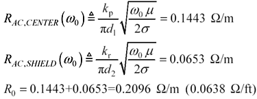
DC resistance (including shield) R DC = 0.0103 W /m (3.14 m W /ft)

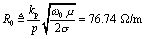
Critical dimension for non-TEM considerations = Shield diameter d 2 = 7.239 mm (0.285 in.)

Conductivity, s = 5.8 ·10 7 S/m

Specification frequency for AC parameters: w = 2 p ·10 7

Characteristic impedance at w : Z = 52 ohms

Effective dielectric constant: R = 2.29

Effective loss tangent for solid polyethylene dielectric: tan q = 0.00052

Proximity factor for 7-way stranded center conductor: k p = 1.07

Surface roughness factor for braided copper shield: k r = 1.8 (applies to frequencies above 10 MHz).

Computed Values

Effective diameter of center conductor: 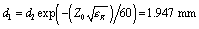(0.077 in.)

Equation 3.147

Propagation velocity above RC region: 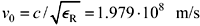( t p =1.54 ns/ft)

Inductance per meter: L = Z / v = 253 nH/m (77.1 nH/ft)

Capacitance per meter: C = 1/( Z v ) = 101 pF/m (30.8 pF/ft)

Lumped-Element Region

Check the critical distance test specified in [3.30] and [3.31]:

Equation 3.148

 

The cable length of l = 2000m well exceeds the critical length. The exit from the lumped-element region will therefore fall along the curve prescribed by [3.26], and the cable will at higher frequencies then proceed to the RC region. Had the length been less than 1262 meters , the cable would have exited the lumped-element region along the curve prescribed by [3.27], transitioning directly into some higher region and bypassing the RC region altogether.

Transitions into all the other major regions are presented in Table 3.11 in units of Hz, which requires an adjustment by a factor of (1/2 p ) from the formulas presented previously in this chapter.

Table 3.11. Onset of Various Transmission Regions (Coaxial Cable Example)

Onset of region	Formula for lower band edge	Value	Source
RC	w LE = ( D / l ) 2 ( R DC C ) “1	2.48 KHz	[3.26]
LC	w LC = ( R DC /L )	6.24 KHz	[3.53]
Skin-effect	w d = w ( R DC / R ) 2	24.1 KHz	[3.104]
Dielectric	w q = (1/ w )[( v R )/( Z tan q )] 2	5.9 GHz	[3.123]
Waveguide (for coax)	w c = 0.586( p v / d 2 )	8 GHz	[3.145]

Operation of this cable at frequencies less than 2.48 KHz may be successfully modeled using a one-stage p network. Above 2.48 KHz a distributed RC model applies until you reach the onset of the LC region at 6.24 KHz. From that point until the skin effect takes hold at 24.1 KHz, the cable response remains fairly flat. Above that the skin effect loss grows in proportion to the square root of frequency until you reach the onset of the dielectric effect at 5.9 GHz. Remember that the transition into the dielectric-loss-limited region is very broad, extending a factor of 100 either side of w q . Well above 5.9 GHz, the loss slope gradually increases until the loss in dB is growing in direct proportion to frequency.

The cable may be successfully operated at frequencies up to nearly 8 GHz without fear of exciting any unusual non-TEM modes of propagation.