Implementation of Frequency-Domain Simulation
The example code in Table 4.2 uses MathCad syntax, although it could easily be rewritten into any mathematical spreadsheet notation. The MathCad symbol := means the variable on the left is assigned the value of the expression on the right.
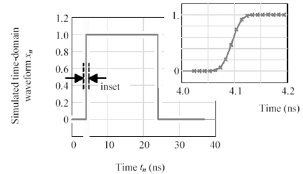
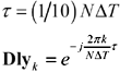
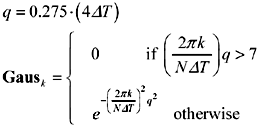
The example in Table 4.2 simulates a pulse of length N /2, with Gaussian rising and falling edges having 10% to 90% rise/fall time equal to 40 ps (4 D T ), and a delay equal to 4096 ps ((1/10) N D T ). These factors were implemented using definitions PulN , Gaus , and Dly from Table 4.1. Such a specification might well represent the differential output of a driver with 1-V amplitude and 40-ps rise/fall time (see Figure 4.4).
Figure 4.4. The time-domain signal x n shows a pulse of length (1/2) N D T , offset by a delay of 4096 ps = (1/10) N D T . The inset reveals a Gaussian rising edge with a 10% to 90% risetime of 40 ps (four samples).
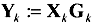
Assuming the differential driver is connected in a system configuration as shown in Appendix C, "Two-Port Analysis," the system gain G may be computed, sampled on the dense grid of frequencies w k to produce a frequency-domain vector G k , and then multiplied point-by-point times the vector X k . The frequency-domain result, once inverse-transformed to the time domain, represents the response of system G to the stimulus X . The time-domain vector y will show the effects of all resistive losses, dielectric losses, bulk transport delay, and reflections within the transmission environment defined by G .
Equation 4.17
Equation 4.18
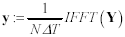
Table 4.2. Example Code Showing FFT Simulation
|
Item |
Expression |
Units |
|---|---|---|
|
Sampling resolution |
D T := 10 “11 |
sec |
|
Length of sample vector |
N := 4096 |
a power of two |
|
Index to time points |
n := 0,1..( N “1) |
integer |
|
Horizontal axis for time-domain plots |
t n := n D T |
sec |
|
Index to frequency points |
k := 0,1..( N /2) |
integer |
|
Horizontal axis for frequency-domain plots |
f k := k/ ( N D T ) |
Hertz |
|
Frequencies used to sample Fourier transform functions |
w k := 2 p f k , k |
rad/sec |
|
Pulse of width ( N/ 2) D T |
|
vector |
|
Delay operator (delays by amount t ) |
|
vector |
|
Gaussian LPF with 10% to 90% rise/fall time equal to 4 D T |
|
vector |
|
Example definition of signal in the frequency domain |
X k := PulN k · Gaus k · Dly k |
vector |
|
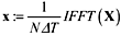
Inverse transformation of frequency-domain vector X to produce time-domain vector x (see Figure 4.4) |
|
vector |
 0,1..( N /2)
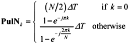
Fundamentals
- Impedance of Linear, Time-Invariant, Lumped-Element Circuits
- Power Ratios
- Rules of Scaling
- The Concept of Resonance
- Extra for Experts: Maximal Linear System Response to a Digital Input
Transmission Line Parameters
- Transmission Line Parameters
- Telegraphers Equations
- Derivation of Telegraphers Equations
- Ideal Transmission Line
- DC Resistance
- DC Conductance
- Skin Effect
- Skin-Effect Inductance
- Modeling Internal Impedance
- Concentric-Ring Skin-Effect Model
- Proximity Effect
- Surface Roughness
- Dielectric Effects
- Impedance in Series with the Return Path
- Slow-Wave Mode On-Chip
Performance Regions
- Performance Regions
- Signal Propagation Model
- Hierarchy of Regions
- Necessary Mathematics: Input Impedance and Transfer Function
- Lumped-Element Region
- RC Region
- LC Region (Constant-Loss Region)
- Skin-Effect Region
- Dielectric Loss Region
- Waveguide Dispersion Region
- Summary of Breakpoints Between Regions
- Equivalence Principle for Transmission Media
- Scaling Copper Transmission Media
- Scaling Multimode Fiber-Optic Cables
- Linear Equalization: Long Backplane Trace Example
- Adaptive Equalization: Accelerant Networks Transceiver
Frequency-Domain Modeling
- Frequency-Domain Modeling
- Going Nonlinear
- Approximations to the Fourier Transform
- Discrete Time Mapping
- Other Limitations of the FFT
- Normalizing the Output of an FFT Routine
- Useful Fourier Transform-Pairs
- Effect of Inadequate Sampling Rate
- Implementation of Frequency-Domain Simulation
- Embellishments
- Checking the Output of Your FFT Routine
Pcb (printed-circuit board) Traces
- Pcb (printed-circuit board) Traces
- Pcb Signal Propagation
- Limits to Attainable Distance
- Pcb Noise and Interference
- Pcb Connectors
- Modeling Vias
- The Future of On-Chip Interconnections
Differential Signaling
- Differential Signaling
- Single-Ended Circuits
- Two-Wire Circuits
- Differential Signaling
- Differential and Common-Mode Voltages and Currents
- Differential and Common-Mode Velocity
- Common-Mode Balance
- Common-Mode Range
- Differential to Common-Mode Conversion
- Differential Impedance
- Pcb Configurations
- Pcb Applications
- Intercabinet Applications
- LVDS Signaling
Generic Building-Cabling Standards
- Generic Building-Cabling Standards
- Generic Cabling Architecture
- SNR Budgeting
- Glossary of Cabling Terms
- Preferred Cable Combinations
- FAQ: Building-Cabling Practices
- Crossover Wiring
- Plenum-Rated Cables
- Laying Cables in an Uncooled Attic Space
- FAQ: Older Cable Types
100-Ohm Balanced Twisted-Pair Cabling
- 100-Ohm Balanced Twisted-Pair Cabling
- UTP Signal Propagation
- UTP Transmission Example: 10BASE-T
- UTP Noise and Interference
- UTP Connectors
- Issues with Screening
- Category-3 UTP at Elevated Temperature
150-Ohm STP-A Cabling
- 150-Ohm STP-A Cabling
- 150- W STP-A Signal Propagation
- 150- W STP-A Noise and Interference
- 150- W STP-A: Skew
- 150- W STP-A: Radiation and Safety
- 150- W STP-A: Comparison with UTP
- 150- W STP-A Connectors
Coaxial Cabling
- Coaxial Cabling
- Coaxial Signal Propagation
- Coaxial Cable Noise and Interference
- Coaxial Cable Connectors
Fiber-Optic Cabling
- Fiber-Optic Cabling
- Making Glass Fiber
- Finished Core Specifications
- Cabling the Fiber
- Wavelengths of Operation
- Multimode Glass Fiber-Optic Cabling
- Single-Mode Fiber-Optic Cabling
Clock Distribution
- Clock Distribution
- Extra Fries, Please
- Arithmetic of Clock Skew
- Clock Repeaters
- Stripline vs. Microstrip Delay
- Importance of Terminating Clock Lines
- Effect of Clock Receiver Thresholds
- Effect of Split Termination
- Intentional Delay Adjustments
- Driving Multiple Loads with Source Termination
- Daisy-Chain Clock Distribution
- The Jitters
- Power Supply Filtering for Clock Sources, Repeaters, and PLL Circuits
- Intentional Clock Modulation
- Reduced-Voltage Signaling
- Controlling Crosstalk on Clock Lines
- Reducing Emissions
Time-Domain Simulation Tools and Methods
- Ringing in a New Era
- Signal Integrity Simulation Process
- The Underlying Simulation Engine
- IBIS (I/O Buffer Information Specification)
- IBIS: History and Future Direction
- IBIS: Issues with Interpolation
- IBIS: Issues with SSO Noise
- Nature of EMC Work
- Power and Ground Resonance
Points to Remember
Appendix A. Building a Signal Integrity Department
Appendix B. Calculation of Loss Slope
Appendix C. Two-Port Analysis
- Appendix C. Two-Port Analysis
- Simple Cases Involving Transmission Lines
- Fully Configured Transmission Line
- Complicated Configurations
Appendix D. Accuracy of Pi Model
Appendix E. erf( )
Notes
EAN: N/A
Pages: 163
- ERP Systems Impact on Organizations
- Challenging the Unpredictable: Changeable Order Management Systems
- Enterprise Application Integration: New Solutions for a Solved Problem or a Challenging Research Field?
- Distributed Data Warehouse for Geo-spatial Services
- Relevance and Micro-Relevance for the Professional as Determinants of IT-Diffusion and IT-Use in Healthcare
