Effect of Inadequate Sampling Rate
Aliasing is the word for the class of problems that result from an inadequate sampling rate. In old Western movies you will sometimes see an extreme form of aliasing cause wagon wheels to turn backwards . This happens because the movie camera takes discrete samples of the wheels at an inadequate rate. If the wheels turn almost one full spoke between each sample, it creates the illusion that the wheels are precessing slowly backwards in successive frames .
In simulations of high-speed digital systems an inadequate sampling rate causes a waveform to "wiggle around" as a function of precisely where it is sampled. For example, suppose you are sampling a continuous-time function with a step at time 1 and a small glitch near time 2.50.
Equation 4.14
Let the sampling interval D T be 1 second. As the samples t n progress through the continuous-time waveform, you get different results depending on where the samples start. For example, samples starting at t = 0 look like this:
Equation 4.15
A train of samples taken starting near t = 0.5, however, would produce this totally different result:
Equation 4.16
Which is correct? The answer, of course, is neither . The waveform defined in [4.14] contains transitions far too quick to be sampled at such a pedestrian rate as 1 sample per second.
Figure 4.3 illustrates the kind of aliasing you are likely to encounter with the frequency-domain simulation if your sampling rate is too slow. This figure shows two rising edges. One is a linear ramp, the other a Gaussian rising waveform. The rise time in both cases is set to 50 ps. The sample interval is 12.5 ps, providing four samples during each rising edge.
Figure 4.3. The Gaussian rising edge displays less wiggling (Gibbs phenomena) than the linear-ramp edge.
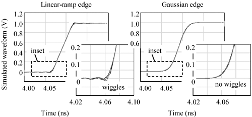
Four frequency-domain simulations are shown. In each simulation the time-domain waveform is sampled and converted to the frequency-domain. The frequency-domain vector is then delayed (using the frequency-domain delay operator) by 1/4, 1/2;, and 3/4; of a sample time. The inverse FFT is then computed for each case, normalized, and the time-domain displays are then successively offset back in time to overlay the original signal. If the sampling rate were infinite, the time-domain shifting would precisely cancel the frequency-domain delay operator, and the waveforms would overlay perfectly . As you can see, they do not.
The linear-ramp edge shows a classic pattern of frequency-domain truncation (Gibbs phenomena) . The limited sampling rate imposes a maximum value on w k , a value which is apparently too small to capture all of the significant high-frequency information present within the signal. The missing high-frequency content induces extraneous wiggles in the signal before and after the rising edge indicating a sensitivity to precisely how the time-domain samples align with the waveform. If you've ever used a scope with an inadequately fast sampling rate, you have probably seen a similar effect ”the sampled waveform appears to "jiggle" on the screen even when you know it contains no jitter.
The figure also shows a Gaussian-rising edge simulated using the same oversampling rate and the same delay procedures. The Gaussian rising edge clearly displays less Gibbs phenomena than the linear-ramp edge. With Gaussian edges an oversampling of 4x the risetime generates a sufficiently dense grid to produce a good representation of the underlying continuous-time signal regardless of the sampling phase alignment.
An FFT theorist would say that the frequency content of the Gaussian-filtered edge is sufficiently suppressed at the Nyquist rate (0.5/ D T Hz) to avoid aliasing.
POINT TO REMEMBER
- In simulations of high-speed digital systems an inadequate sampling rate causes a waveform to "wiggle around" as a function of precisely where it is sampled.
Fundamentals
- Impedance of Linear, Time-Invariant, Lumped-Element Circuits
- Power Ratios
- Rules of Scaling
- The Concept of Resonance
- Extra for Experts: Maximal Linear System Response to a Digital Input
Transmission Line Parameters
- Transmission Line Parameters
- Telegraphers Equations
- Derivation of Telegraphers Equations
- Ideal Transmission Line
- DC Resistance
- DC Conductance
- Skin Effect
- Skin-Effect Inductance
- Modeling Internal Impedance
- Concentric-Ring Skin-Effect Model
- Proximity Effect
- Surface Roughness
- Dielectric Effects
- Impedance in Series with the Return Path
- Slow-Wave Mode On-Chip
Performance Regions
- Performance Regions
- Signal Propagation Model
- Hierarchy of Regions
- Necessary Mathematics: Input Impedance and Transfer Function
- Lumped-Element Region
- RC Region
- LC Region (Constant-Loss Region)
- Skin-Effect Region
- Dielectric Loss Region
- Waveguide Dispersion Region
- Summary of Breakpoints Between Regions
- Equivalence Principle for Transmission Media
- Scaling Copper Transmission Media
- Scaling Multimode Fiber-Optic Cables
- Linear Equalization: Long Backplane Trace Example
- Adaptive Equalization: Accelerant Networks Transceiver
Frequency-Domain Modeling
- Frequency-Domain Modeling
- Going Nonlinear
- Approximations to the Fourier Transform
- Discrete Time Mapping
- Other Limitations of the FFT
- Normalizing the Output of an FFT Routine
- Useful Fourier Transform-Pairs
- Effect of Inadequate Sampling Rate
- Implementation of Frequency-Domain Simulation
- Embellishments
- Checking the Output of Your FFT Routine
Pcb (printed-circuit board) Traces
- Pcb (printed-circuit board) Traces
- Pcb Signal Propagation
- Limits to Attainable Distance
- Pcb Noise and Interference
- Pcb Connectors
- Modeling Vias
- The Future of On-Chip Interconnections
Differential Signaling
- Differential Signaling
- Single-Ended Circuits
- Two-Wire Circuits
- Differential Signaling
- Differential and Common-Mode Voltages and Currents
- Differential and Common-Mode Velocity
- Common-Mode Balance
- Common-Mode Range
- Differential to Common-Mode Conversion
- Differential Impedance
- Pcb Configurations
- Pcb Applications
- Intercabinet Applications
- LVDS Signaling
Generic Building-Cabling Standards
- Generic Building-Cabling Standards
- Generic Cabling Architecture
- SNR Budgeting
- Glossary of Cabling Terms
- Preferred Cable Combinations
- FAQ: Building-Cabling Practices
- Crossover Wiring
- Plenum-Rated Cables
- Laying Cables in an Uncooled Attic Space
- FAQ: Older Cable Types
100-Ohm Balanced Twisted-Pair Cabling
- 100-Ohm Balanced Twisted-Pair Cabling
- UTP Signal Propagation
- UTP Transmission Example: 10BASE-T
- UTP Noise and Interference
- UTP Connectors
- Issues with Screening
- Category-3 UTP at Elevated Temperature
150-Ohm STP-A Cabling
- 150-Ohm STP-A Cabling
- 150- W STP-A Signal Propagation
- 150- W STP-A Noise and Interference
- 150- W STP-A: Skew
- 150- W STP-A: Radiation and Safety
- 150- W STP-A: Comparison with UTP
- 150- W STP-A Connectors
Coaxial Cabling
- Coaxial Cabling
- Coaxial Signal Propagation
- Coaxial Cable Noise and Interference
- Coaxial Cable Connectors
Fiber-Optic Cabling
- Fiber-Optic Cabling
- Making Glass Fiber
- Finished Core Specifications
- Cabling the Fiber
- Wavelengths of Operation
- Multimode Glass Fiber-Optic Cabling
- Single-Mode Fiber-Optic Cabling
Clock Distribution
- Clock Distribution
- Extra Fries, Please
- Arithmetic of Clock Skew
- Clock Repeaters
- Stripline vs. Microstrip Delay
- Importance of Terminating Clock Lines
- Effect of Clock Receiver Thresholds
- Effect of Split Termination
- Intentional Delay Adjustments
- Driving Multiple Loads with Source Termination
- Daisy-Chain Clock Distribution
- The Jitters
- Power Supply Filtering for Clock Sources, Repeaters, and PLL Circuits
- Intentional Clock Modulation
- Reduced-Voltage Signaling
- Controlling Crosstalk on Clock Lines
- Reducing Emissions
Time-Domain Simulation Tools and Methods
- Ringing in a New Era
- Signal Integrity Simulation Process
- The Underlying Simulation Engine
- IBIS (I/O Buffer Information Specification)
- IBIS: History and Future Direction
- IBIS: Issues with Interpolation
- IBIS: Issues with SSO Noise
- Nature of EMC Work
- Power and Ground Resonance
Points to Remember
Appendix A. Building a Signal Integrity Department
Appendix B. Calculation of Loss Slope
Appendix C. Two-Port Analysis
- Appendix C. Two-Port Analysis
- Simple Cases Involving Transmission Lines
- Fully Configured Transmission Line
- Complicated Configurations
Appendix D. Accuracy of Pi Model
Appendix E. erf( )
Notes
EAN: N/A
Pages: 163
