Applying Discrete Fourier Transforms

Problem

You'd like to use a discrete Fourier transform to analyze a dataset but aren't sure how to do so in Excel.

Solution

Use the Fourier Analysis tool in the Analysis ToolPak.

Discussion

Excel provides a Fourier Analysis tool as part of the Analysis ToolPak. This tool allows you to perform discrete Fourier transforms and inverse transforms directly in your spreadsheet. Once your data is transformed, you can manipulate it in either the frequency domain or time domain, as you see fit.

Consider the time series shown in Figure 6-30.

Figure 6-30. Sample time series

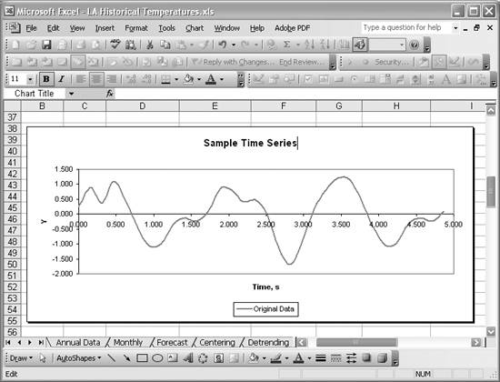
I generated this time series by superimposing several cosine and sine waves of varying frequencies. Discrete samples were taken every 0.15708 (p/20) seconds for a total of 32 samples. Figure 6-31 shows a portion of a spreadsheet containing the data making up this time series.

Figure 6-31. Sample cosine and sine wave frequency data

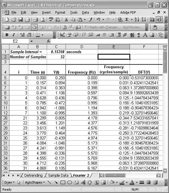
The first column, labeled i, contains an index identifying the sample number. The second column, labeled Time, contains the time at which each sample was taken. And the third column, labeled Y(t), contains the sampled ordinate. There are a total of 32 samples, numbered 0 to 31.

I hid several rows of data in this table so I could fit the first and last rows in one screenshot. You can hide and unhide rows (or columns) by selecting the appropriate menu option from the Format menu. For example, Format images/U2192.jpg border=0> Row images/U2192.jpg border=0> Hide hides the selected row(s).

Before transforming this time series to the frequency domain, I set up a few columns to contain frequency values. A Fourier transform produces the same number of frequency bins, or bands, as time series samples. Therefore, there are 32 frequency bins to label in this example. I used the standard formula fi = i /(ns) to compute the frequencies in cycles per second (Hz), as shown in the Frequency (Hz) column. In this formula, i represents the sample number, n the number of samples, and s the sample interval. The cell formulas in the Frequency (Hz) column are of the form =A5/(n*s). I used cell names (see Recipe 1.14 to learn how to name cells) to name the cells containing the number of samples and the sample interval. Their names are n and s, respectively.

I also computed frequencies in standard units of cycles per sample using the formula fi = i/n. These frequencies are contained in the Frequency (cycles/sample) column. The formulas in this column are of the form =A5/n.

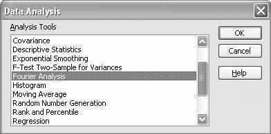
The column DFT(Y) contains the discrete Fourier transform of the time series data. To generate these values you have to use the Fourier Analysis tool. Select Tools images/U2192.jpg border=0> Data Analysis... from the main menu bar to open the Data Analysis dialog box. Select Fourier Analysis from the list of available analysis options shown in Figure 6-32.

Figure 6-32. Fourier Analysis tool selection

Press OK to open the Fourier Analysis dialog box shown in Figure 6-33.

Figure 6-33. Fourier Analysis dialog box

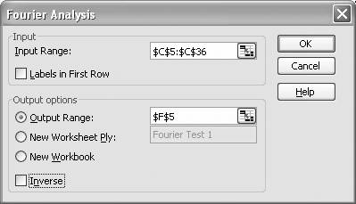
At this point in the example, we're performing a time to frequency domain transform, so make sure the Inverse checkbox is not checked. In the Input Range field, type (or select from your spreadsheet) the cell range containing the time series ordinates to transform. The cell range for this example is C5 to C36. The size of this range must be a power of 2 (for example, 21, 22, 23, 24, and so on). The maximum size is 4,096 (i.e., 212). If your time series data is not a power of 2, then you should pad the end of the series to the next power of 2.

Time series data is often padded on one end before it is transformed, for a couple of reasons. One reason is to build a set of data of a size that's a power of 2. Another reason involves the so-called wraparound effect that can distort results when convolving data. In either case, the padded values of the time series should be 0 if your original time series is centered (see Recipe 6.5). If your time series is not centered, then you can use the average value of the time series ordinates as the pad value. It's also helpful to detrend your time series first if it exhibits a significant trend (see Recipe 6.6).

You have a choice as to where to place the output. You can have the tool place the transformed data on a new worksheet, in which case you supply the name of the new worksheet. Or you can specify a cell on the current worksheet in which to place the results. The results will actually be placed in a column of cells with the specified output cell as the topmost cell. In this example, I specified cell F5 on the current worksheet as the first cell for the output column.

Press OK to close the Fourier Analysis tool and view your results. Column DFT(Y) in Figure 6-31 contains the results for this example. Note that these are complex numbers (you can't see them in their entirety, because I didn't make the cells wide enough). These cell entries look like this: 0.432411242541142-4.7611558001505E-002i. These aren't actually numbers. In fact, they are text. Excel uses text in this form to represent complex numbers. You can still perform mathematical operations on these complex numbers using Excel's complex number worksheet functions. Refer to Recipe 7.13 for a list, along with descriptions, of Excel's built-in complex number functions.

At this point, you have the frequency domain version of your original time series. You can manipulate these results in many different ways to suit the type of analysis you're conducting. For example, you can easily generate a power spectrum of these results to study the frequency content of the original series. All you need to do is add another column to the table shown in Figure 6-31 and use standard formulas for computing the power contained in each frequency band. Figure 6-34 shows a modified table containing a power spectrum calculation for this example.

Figure 6-34. Power spectrum calculation

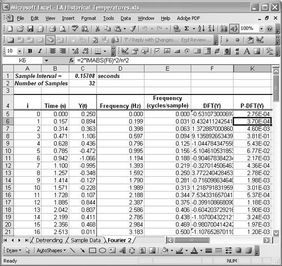
Column P-DFT(Y) is the new one containing the power calculations. These calculations use one of Excel's built-in complex number functions, IMABS, to compute the absolute value of a complex number. For example, the power for the second frequency band, 0.031 cycles/sample, is computed using the cell formula =2*IMABS(F6)^2/n^2. Cell F6 contains the complex number corresponding to a frequency of 0.031 in the discrete Fourier transform data column.

I computed the power for each frequency band up to the highest frequency, the Nyquist frequency (0.5 cycles/sample). The formula used for the power of the 0 frequency band is =IMABS(F5)^2/n^2, while the formula used for the Nyquist frequency band is =IMABS(F21)^2/n^2. The factor of 2 for all intermediate frequency power calculations is due to the periodicity of the Fourier transform and the fact that I'm only computing power from 0 to 0.5 cycles per sample. Figure 6-35 shows a plot of the resulting power spectrum.

Figure 6-35. Power spectrum

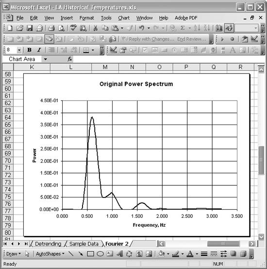
The frequencies on the horizontal axis are in Hz. As you can see, there's a strong component at a frequency of about 0.6 (0.637 to be more specific). Further, there are clear contributions at frequencies of 0.952 and 1.59, though these are not as strong as the one at 0.637.

You can take your analysis even further at this point. Let's say you want to filter the data in the frequency domain to isolate the 0.637 Hz component of the original series. It's relatively easy to construct and apply an appropriate filter in Excel and then perform an inverse Fourier transform to see the resulting filtered series in the time domain.

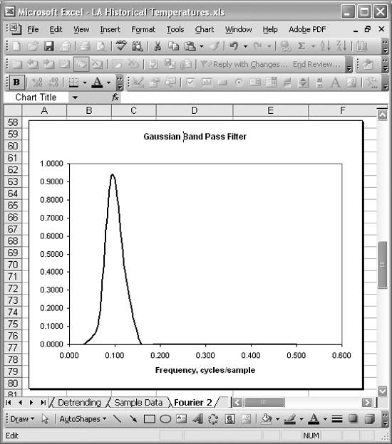
A suitable filter for this example would be a band pass filter centered at a frequency of 0.637 Hz or 0.1 cycles per sample. I used a standard Gaussian band pass filter to calculate the filter values shown in Figure 6-36.

Figure 6-36. Band pass filter calculation

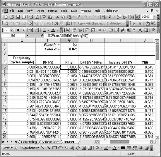
The Filter column contains filter values using formulas of the following form: =EXP(-(((ABS(E5)-fo)/sig)^2)). This equation is a standard Gaussian filter equation. fo is the center frequency, which is contained in cell G1 (I defined the cell name fo to refer to this cell). sig is the spreading factor for the filter, which defines how wide it is in terms of how many frequency bands the filter covers. ABS(E5) is the absolute value of the frequency contained in the column labeled Frequency (cycles/sample). Notice that the center frequency in cell G1 is also expressed in units of cycles per sample.

Figure 6-37 shows a plot of the resulting filter over a frequency range from 0 to 0.5 cycles per sample.

Figure 6-37. Band pass filter

To actually apply this filter, you need to multiply each value in column DFT(Y) by the corresponding value in the Filter column. Remember, however, that the values contained in the DFT(Y) column are actually text values representing complex numbers. Therefore, you have to use one of Excel's built-in complex number functions to perform the multiplication. The appropriate function is the IMPRODUCT function. For example, the cell formulas contained in the column labeled DFT(Y) * Filter in Figure 6-36 are of the form =IMPRODUCT(F5,G5), where the corresponding values in columns DFT(Y) and Filter are used as arguments. The results are complex numbers (text values) contained in the column DFT(Y) * Filter.

At this point, you can construct another power spectrum based on these filtered results to see the relative strength of the frequency components. I generated the filtered power spectrum shown in Figure 6-38 using the same techniques discussed earlier for constructing a power spectrum.

Figure 6-38. Filtered power spectrum

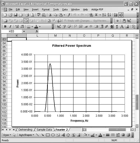
As you can see, this filter effectively isolates the 0.637 Hz frequency component. To see the filtered results back in the time domain, you have to perform an inverse transform.

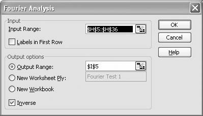
Open the Fourier Analysis tool as explained earlier. Then, referring to Figure 6-36, select the cell range containing the column labeled DFT(Y) * Filter as the input cell range. Select cell I5 as the output cell. Since this is an inverse transform, be sure to check the Inverse checkbox. These settings are shown in Figure 6-39.

Figure 6-39. Inverse transform settings

Press OK when you're done and you should see results that look like those shown in column Inverse DFT(Y) in Figure 6-36. The results of the inverse transform are real numbers in this example; however, Excel formatted them as text (i.e., as the real part of an imaginary number). Use the IMREAL function to convert these imaginary numbers to values you can use. Column Yf(t) in Figure 6-36 contains the results. The cell formulas in that column are of the form =IMREAL(I5).

Now you can plot these filtered results and see how they compare to the original time series. Figure 6-40 shows the comparison.

Figure 6-40. Original versus filtered data

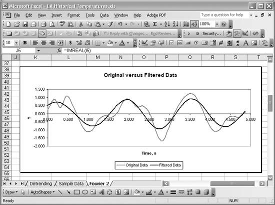
The bold curve shows the filtered time series, where it's clear the high frequency components have been removed.

You can easily replace the band pass filter used in this example with a low- or high-pass filter. For example, the following cell formula creates a low-pass filter: =if(ABS(Ef). Using cell formulas in this manner allows you to construct a wide variety of filters. You can use these same techniques to create window functions if your analysis requires windowing. You can create even more elaborate functions using VBA and call them directly from cell formulas, just as we did the weighted average function in Recipe 6.4.

Chapter 7 Mathematical Functions