Considering Cash Flow Alternatives | Introduction to Financial Calculations

Problem

You're considering two different projects that will generate cash flow streams over a period of years, and each project requires some start-up costs. You want to decide which project offers the highest present value (making it the more attractive option).

Solution

You can set up a cash flow table rather easily using basic spreadsheet functions. Further, you can use the time value of money formulas discussed to discount the future values to present dollars, forming a present value basis of comparison.

Discussion

As an example, let's assume that project A requires an initial outlay of $5,000 during the first year and will generate a positive cash flow of $3,000 per year for the next three years and $4,000 during the fifth year. Project B requires an initial outlay of $6,000 during the first year and will generate a positive cash flow of $3,250 per year for the next three years and $4,250 during the fifth year. We'll assume the time value of money (interest rate) is 4.9%.

If you sum the initial outlay and cash flows for each project, you'll find the sum is $8,000 for each project. Therefore, it would seem they are both equally attractive. However, the story is somewhat different when you consider the time value of money.

What's required is to discount the future cash flow values using the PV function (see Recipe 14.1) to derive cash flow sums for each project in terms of present dollars. Figure 14-1 shows a simple spreadsheet I set up to make these calculations.

Figure 14-1. Discounted cash flow

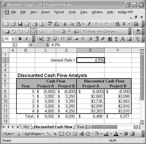
Cell E2 contains the interest rate (4.9%) to be used as the first argument in calls to PV.

Normally, you have to enter percentages in decimal format like 0.049 for 4.9%, 0.1 for 10%, and so on. However, if you format a cell as a percentage (by using Format images/U2192.jpg border=0> Cells ... images/U2192.jpg border=0> Category images/U2192.jpg border=0> Percentage or by entering % after a number in a cell), then you can enter percentages as 4.9, 10, and so on. Excel will take care of the 1/100 factor for you.

The table contained in cells B6 to F13 consists of columns showing the year and cash flow for project A and for project B. The first two cash flow columns are not discounted. The values in these columns were entered manually. The last two cash flow columns are discounted.

The cash flow value for year 0 is not discounted, whereas the cash flows for years 1 through 4 are discounted. The formulas in these cells look like =PV($E$2,$B9,0,-C9,0). The first argument is the interest rate contained in cell E2. The second argument refers to the corresponding year for the particular cash flow value, which is passed in as the fourth argument. I took the negative of the cash flow value so the discounted results come out positive.

The totals in the last row of the table are computed using the SUM formula (see Chapter 7). As it turns out, project A's present value is higher than that of project B. The difference is about 2% and makes project A the more attractive option even though when you look at the nondiscounted cash flows, they both appear to generate the same total cash flow.