Detrending a Time Series

Problem

You're working with a data series that exhibits a clear trend and before processing the data further you need to remove the trend from the data. This is called detrending .

Solution

Construct a trendline in Excel using one of the techniques discussed in Chapter 8 (see Recipe 6.2 for an introduction to trendlines in Excel). Use the resulting trendline to detrend the original data as discussed in this recipe.

Discussion

Time series data is often thought of as being comprised of several components: a long-term trend, seasonal variation, and irregular variations. (Some models assume a fourth, cyclic, component.) When analyzing time series data (e.g., when making forecasts based on historical data), it's often desirable to decompose the time series into its various components. To this end, additive or multiplicative models are often used.

Let Y represent the ordinates of a time series such that Y = f(t), where f is some function of time. Then, we can decompose Y as follows:

or

In these equations, T represents the long-term trend component, S the seasonal component, and I the irregular variation component of the total time series, Y. The first equation is a multiplicative model, while the second is an additive model. Which model you decide to use largely depends on the nature of your data and which model yields the best results. For example, when forecasting you might try both models and use whichever model yields the most accurate predictions. In this and the remaining recipes in this chapter, I'm going to use the multiplicative model; however, you can apply the additive model using very similar Excel techniques.

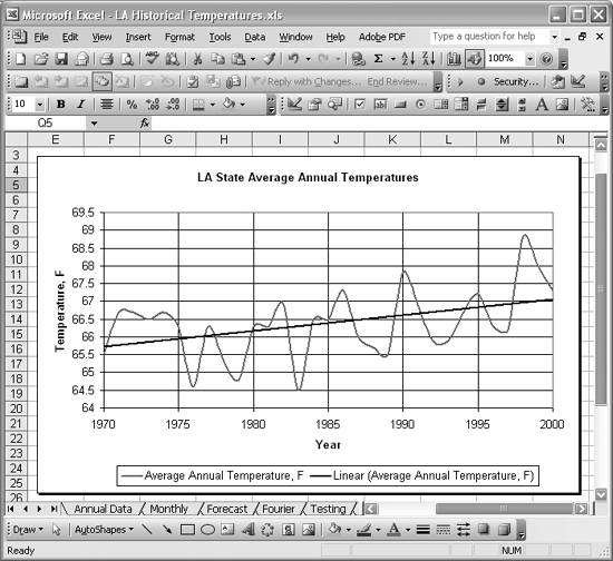
Figure 6-20 shows historical average annual temperatures for the state of Louisiana from 1970 to 2000. This series exhibits a clear upward trend, highlighted by the linear trendline superimposed over the original data.

Figure 6-20. Annual temperatures from 1970 to 2000

If you were going to make a forecast using this historical data, one of the first steps you'd take would be to detrend the original series to remove the long-term trend component.

Using the multiplicative model, divide both sides of the equation Y = TSI by T to yield Y/T = SI. This means the detrended series, Y/T, consists only of the seasonal and irregular variation components. To actually compute Y/T, you must first compute a trendline as shown in Figure 6-20 (see Recipe 6.2 or Chapter 8). Then compute the trend value for each year in the series. Next, divide the original series ordinate (Y) by the computed trend value (T) to yield the detrended series (SI). Figure 6-21 shows a portion of the spreadsheet I set up to perform these calculations for the example temperature series.

Figure 6-21. Detrending example spreadsheet

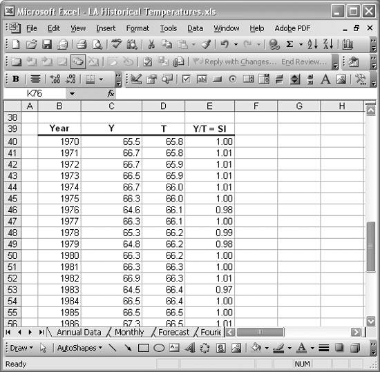
Column B contains the year while column C (under the heading Y), contains the original temperature series.

The formula for the trendline shown in Figure 6-20 is T=0.0446x-22.061, where x is the year. (This trendline equation was determined using Excel's chart trendline feature; see Recipe 6.2.) Column D (under the heading T), contains this formula for each year. The cell formulas in column D are of the form =0.0446*B40-22.061. This series represents the long-term trend component for the original time series.

Finally, column E (under the heading Y/T = SI), contains the detrended series. You simply divide each value in the Y column by the corresponding value in the T column to yield Y/T. The cell formulas in the Y/T = SI column are of the form =C40/D40. Figure 6-22 shows the resulting detrended series.

Figure 6-22. Detrended series

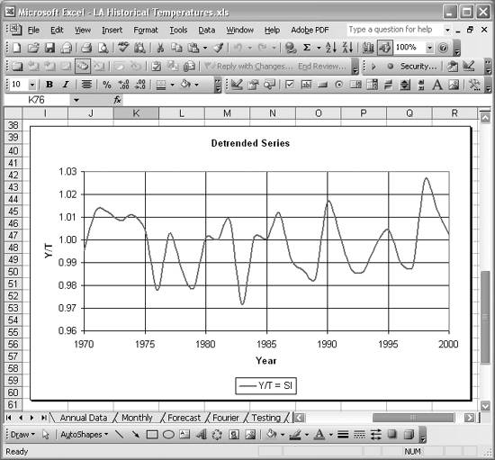
If you were to construct a linear trendline for this series, it would simply consist of a horizontal line. The variations shown in Figure 6-22 are around the long-term trend, and they consist of both seasonal components (if present) and irregular variations. Further analysis (e.g., when forecasting), would probably require you to decompose this series even further to remove the seasonal component. This process is called deseasonalization and is covered in the next two recipes.

See Also

There are other methods of detrending a time series besides using the least squares linear trendline used in this example. Sometimes higher-order trendlines are used, while at other times linear trendlines are computed using only the two series values at each end of the time series. Consult a standard text on time series analysis for more detailed information on these and other detrending methods.