Using Excel for Traditional Linear Programming | Performing Optimization Analyses in Excel

Problem

You've formulated an optimization problem in traditional linear programming form and would like to use Excel to solve the problem.

Solution

Use Solver's linear optimization capabilities.

Discussion

Linear optimization problems can be written in the form of an objective function to maximize (or minimize) subject to constraints. Constraints can be written in the form of inequalities or equalities. Consider this simple example:

Objective function

Constraints

If this were a product mix type of problem, the variables x1 and x2 could represent different products subject to some availability or production constraints, while the objective function could represent total profit given the mix of products produced. The idea is to find the optimum mix of products so as to maximize profit. Linear optimization is not limited to this sort of product mix problem. For example, your problem could consist of trying to maximize the vitamin content of a livestock feed given certain ingredients, subject to their availability and cost. Or your problem could consist of trying to minimize the cost of labor for producing certain products in your laboratory (see the next recipe for a hypothetical example).

Moreover, the problem need not be limited to two variables. You can have any number of variables and constraints, depending on your problem. I chose two variables for this simple example because we can plot it using Excel's charting feature and gain some insight into the solution. Problems with more variables are much more difficult, if not impossible, to visualize adequately. Such problems require you to exercise great care when searching for a solution (particularly if the problem is nonlinear) or to simplify the problem in ways that will allow you to visualize certain variables while holding others constant.

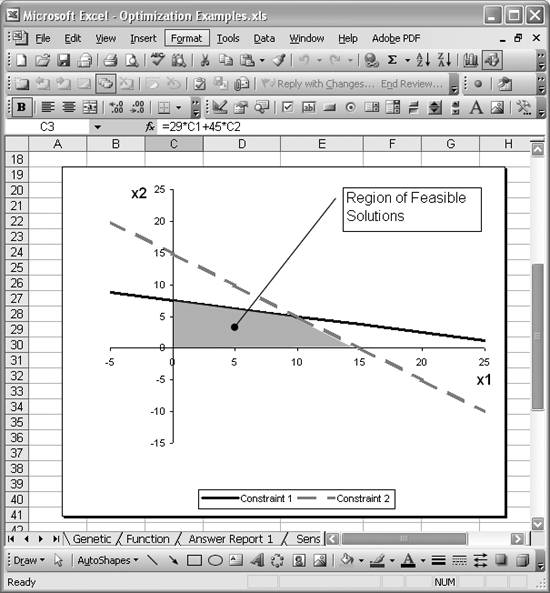
Getting back to our simple example, Figure 13-1 shows a graph of our problem. I used Excel's charting features (see Chapter 4) to prepare this graph.

This graph essentially consists of the constraints for the problem within the x1, x2 space. The two straight lines labeled Constraint 1 and Constraint 2 represent the first two constraints. The shaded region below these constraints represents the region of feasible values for x1 and x2 that are within the given constraints. Notice that this region is bounded by the x1- and x2-axes because we also have the two greater-than-or-equal-to-zero constraints on these variables.

Figure 13-1. Graph of linear optimization example

I drew the shaded region using Excel's AutoShapes Lines images/U2192.jpg border=0> Freeform drawing tool, available from the Drawing toolbar. To draw the shaded area, simply define vertices by pointing and clicking with the mouse. Be sure to select your chart before you start drawing the shaded region, because if you dont, you'll find the resulting shaded region drawn on your spreadsheet, not on your chart. Then when you reposition your chart, you'll find that the shaded area won't move with it.

From this graph, you can deduce that the optimum solution corresponds to (x1,x2) = (10,5), which is at the intersection of the two constraint lines. You can use Solver to verify this result.

Figure 13-2 shows a simple spreadsheet I set up to facilitate finding optimum values for x1 and x2 so as to maximize the objective function.

Figure 13-2. Linear optimization example

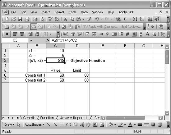
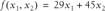
Cell C3 contains the righthand side of the objective function. The formula is =29*C1+45*C2. The values for x1 and x2 shown in Figure 13-2 are indeed the optimum values, and the value of 515 for the objective function is the maximum value. Before calling Solver, cells C1 and C2 contain only initial guesses for the optimum. I had initially set these to 0.

Cells C6 and C7 contain formulas corresponding to Constraint 1 and Constraint 2, respectively. The formula in C6 is =2*C1+8*C2, and the formula in C7 is =4*C1+4*C2. These formulas represent the lefthand side of the constraint equations shown earlier. The limiting values (called righthand side values) for these constraints are contained in cells D6 and D7.

Figure 13-3 shows the Solver model I used to solve this problem.

The target cell is C3 and I instructed Solver to attempt to maximize its value. The cells to change are C1 and C2, corresponding to x1 and x2, respectively. There are four constraints as well. Refer to Recipe 9.4 to learn how to add constraints in Solver.

Figure 13-3. Solver model for linear optimization

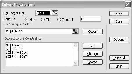
The first two constraints shown in Figure 13-3 correspond to the constraints that x1 and x2 must be greater than or equal to 0. The last two constraints correspond to the constraint equations discussed earlier, that is, Constraint 1 and Constraint 2 as plotted in Figure 13-1.

I also set the Solver option Assume Linear Model for this problem, since it is a linear optimization problem. See the introduction to Chapter 9 for a discussion of Solver's options. Pressing the Solve button results in the optimum solution shown earlier in Figure 13-2.