Shooting Boundary Value Problems

Problem

You need to numerically solve a boundary value problem where you're given an ordinary differential equation and boundary conditions in the problem domain.

Solution

You can use the shooting method to solve the boundary value problem in Excel.

Discussion

The shooting method is a well-known iterative method for solving boundary value problems . Consider this example:

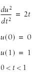
This is a second-order equation subject to two boundary conditions, or a standard two-point boundary value problem .

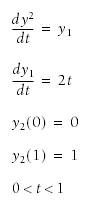
Let y2 = u and y1 = du/dt = dy2/dt to reduce this second-order equation to two first-order equations:

The shooting method attempts to solve this sort of problem as an initial value problem using a marching algorithm like Euler's method or the Runge-Kutta method, as discussed earlier in this chapter. The problem is that the initial conditions are not fully specified; du/dt at t = 0 is unknown. This is the same as saying y1(0) in the reduced system is unknown. Therefore, the shooting method requires you to make an initial guess at the unknown initial condition and then implement a marching algorithm over the problem domain. Once that is complete, you have to check to see if the values obtained at the end of the marching process satisfy the given boundary conditions at the end of the boundary. If they are not satisfied, you have to assume new values for the unknown initial conditions, redo the marching solution, and then check the end boundary conditions again. You repeat this process until you converge on a solution that satisfies all boundary conditions. This iterative process is ideally suited to Excel's Solver tool.

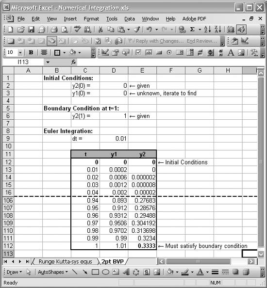
You can readily set this problem up in Excel and solve it using a combination of Solver and a method such as Euler's method. Figure 11-7 shows the spreadsheet I set up to solve the reduced system of equations shown earlier.

At the top of this spreadsheet you can see where I entered the given boundary conditions into several cells. I divided these into initial conditions that will serve as initial conditions for the marching algorithm, and a boundary condition at the end of the problem domain (t = 1). Make sure you notice that the initial condition y1(0) is unknown. The value shown in cell D3 is an assumed initial value. We're going to use Solver to find it later.

The meat of this spreadsheet is the table you see in the middle of Figure 11-7, which implements Euler's method to solve the reduced system of equations. The values at t = 0 in this table contain the initial conditions. For example, the cell containing y1 at t = 0 (cell D12) contains the cell formula =D3, referring back to the unknown initial condition. Similarly, the cell containing y2 at t = 0 (cell E12) contains the cell formula =D2 referring back to the given initial condition.

Figure 11-7. Two-point boundary value problem setup

All of the other cells in this table contain formulas like =D12+2*C13*$D$9 for the y1 column and =E12+D12*$D$9 for the y2 column. These formulas correspond to the Euler integration formulas for this problem shown here:

The table shown in Figure 11-7 is only a portion of the table I set up. You can see that the row labels skip from row 16 to row 106. What happened to the rows in between? I hid them using Format images/U2192.jpg border=0> Row images/U2192.jpg border=0> Hide from the main menu bar (select the rows you want to hide first). This way I could see the bottom end of the table without having to scroll down.

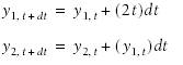
Notice in Figure 11-7 that the computed value for y2 at the end of the domain, t = 1, does not satisfy the given boundary condition. This is because my assumed initial condition, y1(0) = 0, is not the correct initial condition. However, we can use Solver to find it iteratively, subject to the constraint that the value in cell E112 must be equal to the value in cell D6 in order to satisfy the boundary conditions. Figure 11-8 shows the Solver model I set up for this problem.

Figure 11-8. Solver model for two-point boundary value problem

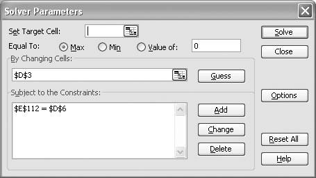
Just as in Recipe 9.4, I didn't specify a target cell. Instead, I specified only a cell to change subject to a single constraint. Solver will automatically set up a dummy target cell if one is not specified. The value of that target cell is irrelevant to the solution. The cell to change for this problem is the value of the unknown initial condition. The constraint consists of requiring the computed value of y2 at the end of the problem domain to equal the given boundary condition. (See Recipe 9.4 to learn how to add constraints in Solver).

Setting up this Solver model and pressing the Solve button starts the iterative solution process, resulting in the solution shown in Figure 11-9.

Figure 11-9. Two-point boundary value problem solution

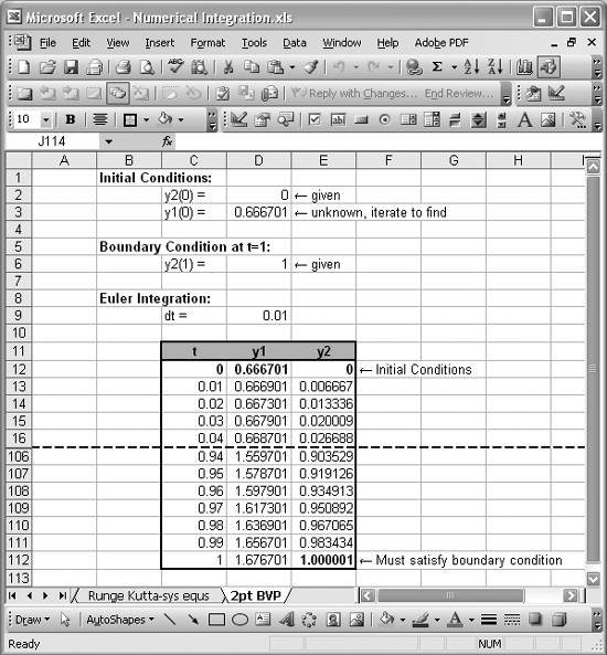
As you can see, Solver found a solution satisfying the specified constraint. It turns out that the correct initial condition for y1 is 0.666701. At this point the problem is solved and you can plot the results if you desire. (See Chapter 4 to learn how to create charts in Excel.)