Introduction

In this chapter we're going to focus on solving equations using Excel. Equation solving, in a general sense, can range from finding roots of single equations, to finding values of independent variables that yield a specific value of a dependent variable, to solving systems of nonlinear equations. There are many traditional hand and computerized methods for solving equations. Newton's method for iteratively finding roots of nonlinear equations and Gaussian elimination with back substitution for solving linear systems are just a couple of examples of classical equation-solving methods. Hildebrand's classic book Introduction to Numerical Analysis presents several classical methods for equation solving. The Numerical Recipes books also present algorithms in a variety of programming languages suitable for equation solving.[*] The methods presented in these and other standard textbooks on numerical methods are just fine and have served scientists and engineers very well. However, in this chapter I want to show you how easy it is to leverage Excel's built-in features to solve equations with very little programming, and in some cases no programming at all beyond basic spreadsheet formulas. After seeing what Excel has to offer, if you still want to program a classic method, I'll show you how to use VBA with Excel to implement a few classic techniques.

[*] See F. B. Hildebrand, Introduction to Numerical Analysis, 2nd ed. (New York: Dover Publications, 1974) and the Numerical Recipes books by Press, Teukolsky, Vetterling, and Flannery, published by Cambridge University Press.

There's not much to gain by using Excel or some other tool to solve equations that can readily be solved by hand after a few algebraic manipulations. Therefore, I'm going to focus almost exclusively on nonlinear equations for the examples presented in this chapter.

I should also add that while most of the example equations are presented in the form of mathematical expressions, this need not be the case for applying the techniques discussed herein. For example, you might have an "equation" composed of several formulas with a few tabular lookups, and so on, that can easily be set up in a spreadsheet. This spreadsheet may then represent a nonlinear equation that you'd like to solve. You can even have calculations span multiple spreadsheets. Ultimately, whether you're dealing with a neat mathematical expression or a complicated spreadsheet, you have both independent variables and dependent variables. Much of what we try to achieve when solving these sorts of equations is finding specific values for the independent variables that yield certain dependent variables. In some cases these dependent variables are indirectly related to the equation being solved, in that we may be trying to find a root for some measure of merit (for example, in least-squares curve fitting).

This sort of calculation also falls within or overlaps the subjects of "what-if" analyses and optimization (see Chapter 13). In both of these cases, you often have to resort to the same iterative techniques used for nonlinear equation solving.

Because the recipes in this chapter rely heavily on the use of Excel's built-in tools Goal Seek and Solver, I want to go over them now to make sure you're aware of their capabilities and differences.

Goal Seek and Solver are handy tools that allow you to easily perform iterative calculations without having to program iterative solution algorithms yourself. For me, these tools are workhorses, and I use them for problems ranging from solving nonlinear systems of equations to optimization analysis to forecasting. I've even used Solver to solve the equations of motion for a hydrofoil boat that I built and tested.

On the surface it appears as though Goal Seek and Solver do the same thing; that is, they both allow you to iteratively find a target value in a target cell by changing a value in some other related cell. There are, however, certain key differences between Goal Seek and Solver that you should be aware of when deciding which tool to use for a particular problem. The discussion to follow describes these key differences.

Goal Seek

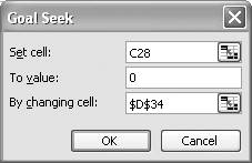
Goal Seek is quick and simple to use. Simply specify a target value for a target cell and specify the independent cell to vary in order to reach the target. Figure 9-1 shows Goal Seek's interface. (You can access Goal Seek from the Tools menu; select Tools images/U2192.jpg border=0> Goal Seek...from the main menu bar.)

The "Set cell" field contains the target cell whose value you want to set to the value contained in the "To value" field. You tell Goal Seek which cell to change by specifying a cell in the "By changing cell" field. The target cell must contain a formula that must also directly or indirectly refer to the cell specified in the "By changing cell" field.

Figure 9-1. Goal Seek window

You can also use Goal Seek from within VBA subroutines, so you don't have to access it manually. This comes in handy when you need to use Goal Seek repeatedly. See Recipe 9.3 for an example.

You can vary only one cell using Goal Seek; thus Goal Seek is only for univariate problems. Further, you must specify the target value explicitly; that is, you have to give a numerical value as the target value. Also, Goal Seek does not allow you to impose any constraints on the independent cell (the cell in the "By changing cell" field).

According to a short article on Microsoft's support web site (Article ID 100782), Goal Seek employs a linear search algorithm using initial guesses around the value initially set in the independent cell. This means that the value contained in the independent cell when you first start Goal Seek in effect serves as your initial guess. This is important to remember, especially when solving problems with more than one solution. For example, if you're trying to find the roots of a cubic equation, your initial guess may result in Goal Seek converging on one solution, while a different initial guess will result in convergence on the other solution. This also implies that if Goal Seek fails to converge on a solution, you should try a different initial guess.

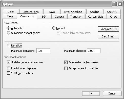
Goal Seek considers convergence successful if the maximum amount of change between iterations falls below some threshold. By default, this threshold is 0.001. Goal Seek will also stop if the number of iterations exceeds some maximum (100 by default). You can change these criteria by selecting Tools images/U2192.jpg border=0> Options...from the main menu bar, which opens the Options window as shown in Figure 9-2.

Click the Calculation tab to reveal the calculation options. Toward the middle of the window you'll see an Iteration checkbox along with "Maximum iterations" and "Maximum change" fields. Specify appropriate values in these fields and check the Iteration checkbox so they take effect.

For simple iterative problems, Goal Seek is quite capable and it's quick and easy to use. However, for more complex problems or where more control over the iterative process is required, Solver is the tool of choice.

Figure 9-2. Options window

 

Solver

Solver is similar to Goal Seek in that you can iteratively find a target value in a target cell by changing values in an independent cell, but Solver's features go well beyond those of Goal Seek. This is reflected in the more complex interface to Solver, which is shown in Figure 9-3. (You can access Solver from the Tools menu. If you don't see it listed there, go to Tools images/U2192.jpg border=0> Add-Ins...and select Solver Add-in to make it available; then go to Tools images/U2192.jpg border=0> Solver...to open it.)

Figure 9-3. Solver Parameters window

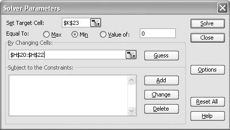
You can use Solver for multivariate problems, where you want to vary more than one independent cell to obtain some target value in a target cell. You can specify the cells to vary in the By Changing Cells field . You can use any valid cell reference format here, with multiple cell references separated by commas. In the version of Solver that's bundled with Excel, you can select up to 200 cells to change.

You can use the Guess button to let Solver attempt to "guess" the independent cells to change for your problem. I usually shy away from this feature, though. All it does is select all nonformula cells that are referred to by the formula contained in the target cell. For simple formulas with a few independent variables where you want to change them all, this may be useful. However, for the problems I've encountered I find it selects way too many cells, many of which I don't want to vary at all (e.g., certain constants or values that I want to fix for one reason or another). On the other hand, if you're dealing with a large number of variables, it might be easier to let Solver select them all and then manually remove the ones you don't want from the By Changing Cells field.

In Solver you don't even have to specify a target value. Instead you can choose to maximize or minimize the value in the target cell. The target cell is referred to in the Set Target Cell field (it must be a single cell that contains a formula). The Equal To radio buttons allow you to specify whether to maximize or minimize the target cell or set its value to a specific numerical value.

Solver does not stop there. You can even specify constraints on cells that are part of the problem being solved. These constraints allow you to impose equalities or upper and lower bounds on values within cells. This is a handy feature when you're trying to bracket a solution or when performing constrained optimization problems. Recipe 9.4 shows how to use constraints with Solver to solve simultaneous equations. Also, Chapter 13 contains recipes on using Solver for constrained optimization. Solver allows up to 100 constraints for nonlinear problems and up to 200 constraints for linear problems (in the version that's bundled with Excel).

Solver also has more available solution algorithms than does Goal Seek. For linear problems, Solver uses the simplex method. Solver is also capable of handling nonlinear problems by employing a generalized reduced gradient method. In cases where the problem being solved requires integer-valued variables, Solver also employs a branch and bound algorithm.

You do have a little control over these algorithms in Solver via the Options window. Press the Options button on the Solver Parameters window to display the Solver Options window (see Figure 9-4).

Figure 9-4. Solver Options window

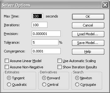
As you can see, there are several more options here, as opposed to the two available for Goal Seek. Solver's options include:

 

Max Time

Max Time represents the maximum amount of time to allow Solver to obtain a solution, after which the process will be aborted. Solver will display a message box saying that it could not find a solution within the allowable time. You can set this value as high as 32,767 seconds (just over 9 hours), though I doubt you'll ever have to do so.

 

Iterations

Iterations specifies the maximum number of iterations to allow Solver while attempting to find a solution. If the maximum number of iterations is reached before Solver finds a solution, the process will be aborted and Solver will display a message box saying that it could not find a solution within the allowable number of iterations. You can set this value as high as 32,767, though in my experience I've never had to set it above 1,000 and usually leave it at the default value of 100.

 

Precision

Precision is specified as a decimal number between 0 and 1, with a default value of 1.0 x 10-6. It is used by Solver to determine when a constraint is satisfied. The lower the value specified here, the higher the precision. Rarely do I have to change this value in practice.

 

Tolerance

Tolerance is used to determine whether or not an integer-valued constraint is satisfied. Tolerance is expressed as a percentage, with a default value of 5%. If you're not using integer constraints, then Tolerance does not apply.

 

Convergence

Convergence is used to determine whether or not Solver has converged on a solution. Solver considers a solution converged upon when the optimal values are within the value specified in the Convergence field over the last five solution iterations. Solver will display a message box after it converges on a solution. Solver will continue trying to converge so long as the specified maximum number of iterations or maximum time has not been reached. If either limit is reached, Solver will display a message box indicating that it could not converge.

 

Assume Linear Model

In cases where you know your problem consists of a linear model you can specifically instruct Solver to use the simplex method of solution rather than the generalized reduced gradient method. In the event that you do specify this option, Solver will perform some checks to see if your model is indeed linear according to its criteria. If not, a message box will appear, warning you that your model does not fit the criteria for a linear model.

 

Assume Non-Negative

You can check this to instruct Solver to automatically set lower limit constraints on all variable cells. If you know that your variables should always be greater than 0 and you want to constrain them to be so, check this option. This way you can avoid having to add a constraint manually for each variable.

 

Use Automatic Scaling

In some problems the values of the independent variables and dependent variables may differ widely in magnitude. In these cases it's prudent to scale the model so that the magnitudes of the input and output values are of the same order. If you didn't already set up your model with scaling, then you can select this option to allow Solver to perform the scaling for you. In this case, it will scale your input and output values by dividing them by the initial value specified in the variable and target cells. This makes your initial guesses extra important for problems where scaling is required. It is always best to set your initial values to something realistic and reasonable for the problem under consideration.

 

Show Iteration Results

If you want to follow Solver's progress as it iterates when solving a problem, you can check the Show Iteration Results option. When you do, a dialog box will appear, saying that Solver is paused and that the current iteration's results are displayed on the active worksheet. This option is useful when you want to see the results of each iteration step; for example, when Solver can't find a solution, you can use this option to try to gain insight as to why not. Under normal circumstances I do not check this option, since you actually have to press a button each time Solver is paused in order for it to proceed to the next step. This can become tedious if the solution for a particular problem requires much iteration.

 

Estimates

Here you can specify how Solver will estimate initial values of the independent variables. Tangent uses linear extrapolation, whereas Quadratic uses quadratic extrapolation and is said to speed convergence for nonlinear problems. Quite frankly, given today's high-speed processors, I notice little difference on convergence time for typical problems.

 

Derivatives

Solver uses finite differences to compute gradients and provides two options for your control. You can use either a forward differencing scheme or a central differencing scheme. Central differencing requires more computations but is generally more accurate. Here again, the difference in processing time using either method may be imperceptible on today's processors. I generally just use central differencing. (See Recipe 10.6 for more discussion on forward differencing versus central differencing in general numerical work.)

 

Search

You can choose to instruct Solver to use either Newton's method or the conjugate gradient method for solving a problem. Solver uses these methods to determine search directions during each iteration. Newton's method requires fewer computations than the conjugate method; however, Newton's method requires more memory. If memory is a concernfor example, if you're dealing with a very large problem with many variables and constraints or if your computer memory is limitedthen you might want to use the conjugate method.

There are two other available Solver options that don't affect the solution process for Solver, though they are useful nonetheless. These options are Load Model and Save Model. Basically, Solver allows you to save Solver models and reload them. This can be quite handy when you're trying different combinations of variables and constraints along with solution options to see which model works best for a given problem. It also allows you to recall a model later (without having to remember all the model settings) if you decide to come back and redo an analysis.

Press the Save Model button to save a model. When you do, a small dialog box will appear, asking you to select a range of cells within which the model data will be saved. You should select a range of cells away from other data and formulas in your spreadsheet so that you don't overwrite anything. You need only select a single cell and Solver will fill in a column of data, starting with the selected cell, consisting of a number of cells totaling 3 plus the number of constraints in your model.

To recall a model later, simply go to the Solver Options window and press the Load Model button. You will then see a small dialog box asking you to select the range of cells containing the saved model. You must select the entire range of cells previously saved. Selecting only the uppermost cell will not work.

Another handy Solver feature not included with Goal Seek is the Solver Results feature. Upon finding a solution, Solver will notify you via a message box like that shown in Figure 9-5.

Figure 9-5. Solver Results window

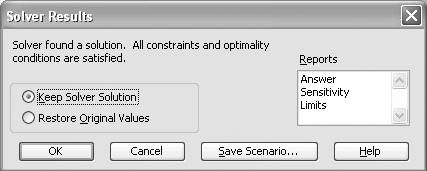
Here you can choose to keep the solution found by Solver, or revert back to your original values. Moreover, you can choose to generate any of three Solver reports: Answer, Sensitivity, or Limits. Click on each report name that you want. You can click one or all or any combination. When you press the OK button, Solver will create a new worksheet for each selected report. These reports are useful for interpreting the results of a Solver solution, particularly for constrained optimization problems. I talk more about these reports in Chapter 13, which covers optimization.

You can always refer to the Solver help documents in Excel by pressing the help buttons that appear on the various Solver-related windows. For more interesting reading about the history and inner workings of Solver, check out the paper "Design and Use of the Microsoft Excel Solver," by Daniel Fylstra, Leon Lasdon, John Watson, and Allan Waren, published in Interfaces 28, no. 5 (1998).