Recruiting Solver to Iteratively Solve Finite Difference Equations
Problem
You've set up a finite difference solution to an elliptic boundary value problem, but instead of directly solving a system of algebraic equations, you want to use an iterative approach.
Solution
Set up your finite difference equations in Excel and use Solver to iteratively find a solution.
Discussion
In Recipe 12.1, I explained how you can use Excel's matrix functions to directly solve systems of finite difference equations. For small systems, direct matrix operations are viable; however, for large systems the use of matrix functions in Excel is cumbersome. Other standard direct methods include Gauss elimination and Fourier's method, among others. These methods could be programmed in Excel; however, there's another class of methods known as iterative methods that are more attractive.
Iterative solutions to finite differences equations abound. Various standard methods such as Jacobi's method , Gauss-Seidel iteration (also called Liebmann's method ), and the alternating direction implicit (ADI) method are commonly used in lieu of direct methods. Iterative methods have an advantage over direct methods in that they typically require less memory and are relatively easy to program. Moreover, when using Excel to help solve your problem, you already have access to a powerful iterative tool, Solver. This means that you can use Solver to find a solution to your finite difference equations without any programming beyond setting up a spreadsheet.
By way of example, consider the steady state temperature distribution in a square plate. The left, right, and bottom edges of the plate are maintained at a constant 100°C, whereas the top of the plate is maintained at a constant 0°C. The temperature distribution in the interior of the plate is governed by the Laplace equation shown earlier, where u represents temperature. The Laplace equation is repeated here for convenience:

A finite difference mesh for this problem might look something like that shown in Figure 12-2.
Figure 12-2. Finite difference grid for temperature distribution in square plate
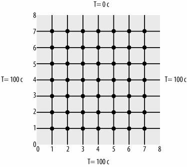
Each little circle shown in the grid in Figure 12-2 represents a computational node where the following finite difference equation, from the previous recipe, applies:

In this example, I'm assuming the grid spacing, h, is uniform in both x and y directions and equal to 1 cm.
If you rearrange this finite difference equation, solving for u(x, y), you get the following:

You can see that u (the temperature) at each node is simply the average of the temperatures of adjacent nodes. For nodes adjacent to the plate boundary, the specified boundary conditions are included in the average.
This example results in 49 finite difference equations with 49 unknown temperatures. A temperature distribution is sought that satisfies the above equation at each node.
Another way to look at this problem is to reconsider this form of the finite difference equation:

This is the same equation shown earlier, prior to solving for u(x, y). This form of the equation represents the residual at each nodethat is, the temperature minus the estimated temperature at each node. This residual must ideally be 0. If you take all these residuals, one for each node, and square them and then sum the squares, you end up with a least-squares minimization problem. You can use Solver to minimize the sum of squared residuals to arrive at a solution that satisfies the governing equations. Figure 12-3 shows the spreadsheet I set up to solve this problem in Excel.
Figure 12-3. Finite difference spreadsheet setup
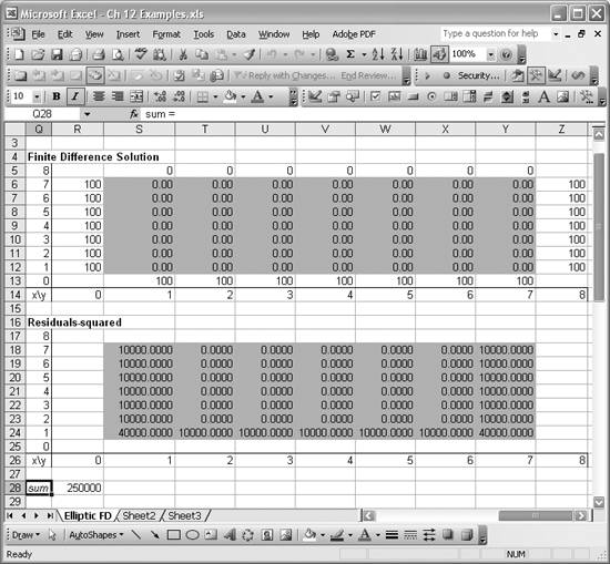
The table under the heading Finite Difference Solution represents the temperature distribution satisfying the governing equations and boundary conditions. At the moment, the table is filled with initial guesses except at the boundaries, where the given boundary conditions are applied. Each of the shaded cells in this table corresponds to a computational node in the finite difference grid illustrated in Figure 12-2. The nonshaded cells bounding the shaded cells correspond to boundary nodes with specified boundary conditions.
The lower table in Figure 12-3, under the heading Residuals-squared, contains a similar set of shaded cells. In this case, the shaded cells contain the finite difference equation for each node, squared. The cell formulas are of the following form: =(-4*S6+S5+S7+R6+T6)^2. This is the cell formula for cell S18. All the other cells contain similar formulas with relative cell references. This form is essentially the square of the residual for each node. Note that these formulas refer to the values for each node contained in the upper table.
Cell R28 contains the formula =SUM(S18:Y24). This is simply the sum of all squared residuals contained in the lower table.
Now you can use Solver to minimize the value in cell R28 by changing all the values contained in the shaded cells in the upper table. Figure 12-4 shows the Solver model I used for this example.
Figure 12-4. Solver model for finite difference solution
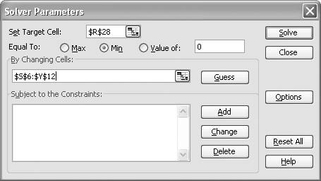
You can see that this model aims to minimize the value in cell R28, the sum of squared residuals, by changing all the values contained in cells S6 to Y12. If Solver is successful, cells S6 to Y12 in the upper table in Figure 12-3 will contain a temperature distribution that satisfies the governing equations and boundary conditions.
After you press the Solve button, Solver does indeed find a solution, as shown in Figure 12-5.
Figure 12-5. Solution to finite difference problem
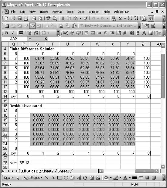
As you can see, the sum of squared residuals is a very small number and the squared residuals for each cell are all 0 (to 14 decimal places). The upper table now contains the solution to the temperature distribution problem.
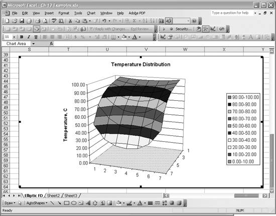
Just for fun, I plotted these results using Excel's 3-D Surface chart feature (see Chapter 4). Figure 12-6 shows the resulting plot.
This highlights another advantage of using Excel: you can quickly visualize your results without having to program your own visualizations or use a separate visualization tool.
Figure 12-6. Surface plot of temperature distribution
Using Excel
- Introduction
- Navigating the Interface
- Entering Data
- Setting Cell Data Types
- Selecting More Than a Single Cell
- Entering Formulas
- Exploring the R1C1 Cell Reference Style
- Referring to More Than a Single Cell
- Understanding Operator Precedence
- Using Exponents in Formulas
- Exploring Functions
- Formatting Your Spreadsheets
- Defining Custom Format Styles
- Leveraging Copy, Cut, Paste, and Paste Special
- Using Cell Names (Like Programming Variables)
- Validating Data
- Taking Advantage of Macros
- Adding Comments and Equation Notes
- Getting Help
Getting Acquainted with Visual Basic for Applications
- Introduction
- Navigating the VBA Editor
- Writing Functions and Subroutines
- Working with Data Types
- Defining Variables
- Defining Constants
- Using Arrays
- Commenting Code
- Spanning Long Statements over Multiple Lines
- Using Conditional Statements
- Using Loops
- Debugging VBA Code
- Exploring VBAs Built-in Functions
- Exploring Excel Objects
- Creating Your Own Objects in VBA
- VBA Help
Collecting and Cleaning Up Data
- Introduction
- Importing Data from Text Files
- Importing Data from Delimited Text Files
- Importing Data Using Drag-and-Drop
- Importing Data from Access Databases
- Importing Data from Web Pages
- Parsing Data
- Removing Weird Characters from Imported Text
- Converting Units
- Sorting Data
- Filtering Data
- Looking Up Values in Tables
- Retrieving Data from XML Files
Charting
- Introduction
- Creating Simple Charts
- Exploring Chart Styles
- Formatting Charts
- Customizing Chart Axes
- Setting Log or Semilog Scales
- Using Multiple Axes
- Changing the Type of an Existing Chart
- Combining Chart Types
- Building 3D Surface Plots
- Preparing Contour Plots
- Annotating Charts
- Saving Custom Chart Types
- Copying Charts to Word
- Recipe 4-14. Displaying Error Bars
Statistical Analysis
- Introduction
- Computing Summary Statistics
- Plotting Frequency Distributions
- Calculating Confidence Intervals
- Correlating Data
- Ranking and Percentiles
- Performing Statistical Tests
- Conducting ANOVA
- Generating Random Numbers
- Sampling Data
Time Series Analysis
- Introduction
- Plotting Time Series Data
- Adding Trendlines
- Computing Moving Averages
- Smoothing Data Using Weighted Averages
- Centering Data
- Detrending a Time Series
- Estimating Seasonal Indices
- Deseasonalization of a Time Series
- Forecasting
- Applying Discrete Fourier Transforms
Mathematical Functions
- Introduction
- Using Summation Functions
- Delving into Division
- Mastering Multiplication
- Exploring Exponential and Logarithmic Functions
- Using Trigonometry Functions
- Seeing Signs
- Getting to the Root of Things
- Rounding and Truncating Numbers
- Converting Between Number Systems
- Manipulating Matrices
- Building Support for Vectors
- Using Spreadsheet Functions in VBA Code
- Dealing with Complex Numbers
Curve Fitting and Regression
- Introduction
- Performing Linear Curve Fitting Using Excel Charts
- Constructing Your Own Linear Fit Using Spreadsheet Functions
- Using a Single Spreadsheet Function for Linear Curve Fitting
- Performing Multiple Linear Regression
- Generating Nonlinear Curve Fits Using Excel Charts
- Fitting Nonlinear Curves Using Solver
- Assessing Goodness of Fit
- Computing Confidence Intervals
Solving Equations
- Introduction
- Finding Roots Graphically
- Solving Nonlinear Equations Iteratively
- Automating Tedious Problems with VBA
- Solving Linear Systems
- Tackling Nonlinear Systems of Equations
- Using Classical Methods for Solving Equations
Numerical Integration and Differentiation
- Introduction
- Integrating a Definite Integral
- Implementing the Trapezoidal Rule in VBA
- Computing the Center of an Area Using Numerical Integration
- Calculating the Second Moment of an Area
- Dealing with Double Integrals
- Numerical Differentiation
Solving Ordinary Differential Equations
- Introduction
- Solving First-Order Initial Value Problems
- Applying the Runge-Kutta Method to Second-Order Initial Value Problems
- Tackling Coupled Equations
- Shooting Boundary Value Problems
Solving Partial Differential Equations
- Introduction
- Leveraging Excel to Directly Solve Finite Difference Equations
- Recruiting Solver to Iteratively Solve Finite Difference Equations
- Solving Initial Value Problems
- Using Excel to Help Solve Problems Formulated Using the Finite Element Method
Performing Optimization Analyses in Excel
- Introduction
- Using Excel for Traditional Linear Programming
- Exploring Resource Allocation Optimization Problems
- Getting More Realistic Results with Integer Constraints
- Tackling Troublesome Problems
- Optimizing Engineering Design Problems
- Understanding Solver Reports
- Programming a Genetic Algorithm for Optimization
Introduction to Financial Calculations
- Introduction
- Computing Present Value
- Calculating Future Value
- Figuring Out Required Rate of Return
- Doubling Your Money
- Determining Monthly Payments
- Considering Cash Flow Alternatives
- Achieving a Certain Future Value
- Assessing Net Present Worth
- Estimating Rate of Return
- Solving Inverse Problems
- Figuring a Break-Even Point
Index
EAN: 2147483647
Pages: 206
