Tackling Coupled Equations

Problem

You've seen how to apply both the Runge-Kutta method and Euler's basic method using VBA for first- and second-order differential equations, but now you need to solve a system of coupled equations . You're wondering how to extend what you've learned so far to deal with this more complicated problem.

Solution

You can apply the same VBA techniques discussed earlier with some modifications to deal with multiple equations.

Discussion

Consider this system of coupled nonlinear differential equations with initial conditions:

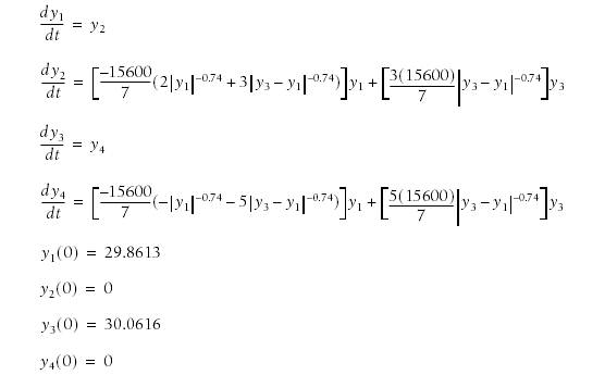
Pretty, huh? This problem originally consisted of two coupled second-order equations that were reduced to four first-order equations using the same technique discussed in Recipe 11.2. This is a common technique for reducing the order of differential equations, making them more amenable to solving. This particular problem was adapted from a problem that appears in An Introduction to Linear and Nonlinear Finite Element Analysis, by Prem K. Kythe and Dongming Wei (Birkhauser). The problem represents a finite element solution of the nonlinear vibrations of a metal rod. Since this is a nonlinear problem, it requires a numerical solution. In their book, Kythe and Wei present some Matlab code to solve this problem using Euler's method .

Euler's method

I implemented Euler's method in VBA to illustrate how to solve this same system in Excel. Example 11-4 shows my VBA code.

Example 11-4. DoEuler for nonlinear system

Public Sub DoEuler( )
 Dim y(1 To 4) As Double
 Dim t(1 To 4) As Double
 Dim n As Integer
 Dim dt As Double
 Dim time As Double
 
 y(1) = 29.8613
 y(2) = 0
 y(3) = 30.0616
 y(4) = 0
 
 n = 5000
 dt = 5 / n
 time = 0
 
 For i = 1 To n
 t(1) = y(1) + dt * dy1dt(y(1), y(2), y(3), y(4))
 t(2) = y(2) + dt * dy2dt(y(1), y(2), y(3), y(4))
 t(3) = y(3) + dt * dy3dt(y(1), y(2), y(3), y(4))
 t(4) = y(4) + dt * dy4dt(y(1), y(2), y(3), y(4))
 
 y(1) = t(1)
 y(2) = t(2)
 y(3) = t(3)
 y(4) = t(4)
 
 time = time + dt
 ActiveSheet.Cells(i + 1, 1) = time
 ActiveSheet.Cells(i + 1, 2) = y(1)
 ActiveSheet.Cells(i + 1, 3) = y(2)
 ActiveSheet.Cells(i + 1, 4) = y(3)
 ActiveSheet.Cells(i + 1, 5) = y(4)
 Next i
End Sub

As you can see, this is not a particularly complicated subroutine. It's very similar to the code in Example 11-2 that I showed you for solving a first-order equation using Euler's method. The major difference in this case is that we have four coupled equations instead of a single equation.

I'm using VBA array variables in this code for the y-values and temporary t-values. In VBA, you declare an array using Dim y(1 To 4) As Double. You can access the array using y(1) or y(3), and so on.

I have to confess that there's a little more to this code than is shown in Example 11-4. Notice the function callsdy1dt, dy2dt, dy3dt, dy4dtin the lines of code that implement Euler's integration formula (the lines just after the For statement). These functions compute the derivatives for each y. The derivative expressions are taken directly from the system of equations shown earlier. The corresponding VBA functions are shown in Example 11-5.

Example 11-5. Derivative functions

Public Function dy1dt(y1 As Double, y2 As Double, y3 As Double, y4 As Double) As Double
 dy1dt = y2
End Function
 
Public Function dy2dt(y1 As Double, y2 As Double, y3 As Double, y4 As Double) As Double
 dy2dt = (-15600# * (2# * ((Abs(y1)) ^ -0.74) + 3# * ((Abs(y3 - y1))^-0.74))) _
 / 7# * y1 + (3# * 15600# * ((Abs(y3 - y1)) ^ -0.74)) / 7# * y3
End Function
 
Public Function dy3dt(y1 As Double, y2 As Double, y3 As Double, y4 As Double) As Double
 dy3dt = y4
End Function
 
Public Function dy4dt(y1 As Double, y2 As Double, y3 As Double, y4 As Double) As Double
 dy4dt = (-15600# * (-((Abs(y1)) ^ -0.74) - 5# * ((Abs(y3 - y1)) ^ -0.74))) _
 / 7# * y1 - (5# * 15600# * ((Abs(y3 - y1)) ^ -0.74)) / 7# * y3
End Function

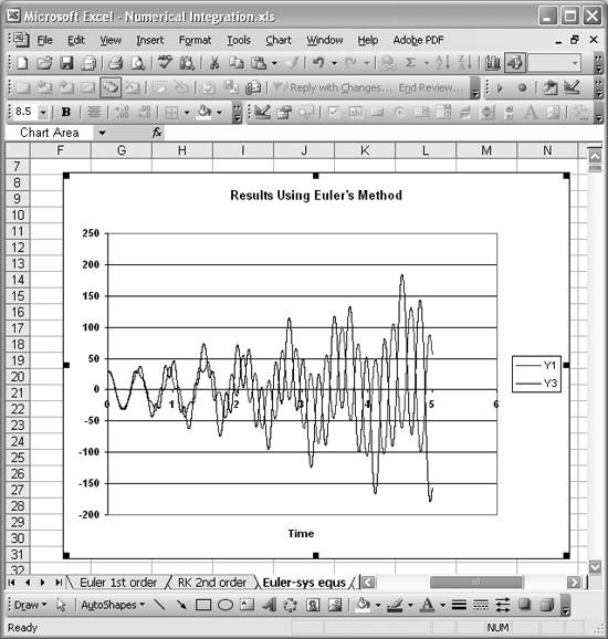
This code runs just fine. The problem is that this is a particularly troublesome system of equations for Euler's method. The solution diverges dramatically as it marches along in time. Check out Figure 11-5 to see what I mean.

The chart shows y1 and y3the displacements of the rod at its center and free endover time. The results should look sinusoidal. However, you can clearly see that this solution is not a sinusoid. This is wonderful example of the sort of problem where Euler's method, though easy to implement, is a poor choice.

Runge-Kutta method

The Runge-Kutta method presents a better alternative to Euler's method for this problem. In Recipe 11.2, I showed you how to reduce a second-order equation to two first-order equations and then use the Runge-Kutta method to solve one and use a Euler step to solve the other. In this new example, I'll show you how to apply the Runge-Kutta method for all four equations at each time step. To this end, I prepared a new subroutine, DoRungeKutta, shown in Example 11-6. DoRungeKutta also makes calls to the derivative functions shown earlier in Example 11-5.

Figure 11-5. Poor results using Euler's method

 

Example 11-6. Runge-Kutta for nonlinear system

Public Sub DoRungeKutta( )
 ' Declar Local variables
 Dim y(1 To 4) As Double
 Dim k1(1 To 4) As Double
 Dim k2(1 To 4) As Double
 Dim k3(1 To 4) As Double
 Dim k4(1 To 4) As Double
 Dim n As Integer
 Dim dt As Double
 Dim time As Double
 
 Application.ScreenUpdating = False
 
 ' Initialize variables
 y(1) = 29.8613
 y(2) = 0
 y(3) = 30.0616
 y(4) = 0
 n = 5000
 dt = 5 / n:
 time = 0
 
 ' Perform iterations
 For i = 1 To n
 k1(1) = dt * dy1dt(y(1), y(2), y(3), y(4))
 k1(2) = dt * dy2dt(y(1), y(2), y(3), y(4))
 k1(3) = dt * dy3dt(y(1), y(2), y(3), y(4))
 k1(4) = dt * dy4dt(y(1), y(2), y(3), y(4))
 
 k2(1) = dt * dy1dt(y(1)+k1(1)/2#, y(2)+k1(2)/2#, y(3)+k1(3)/2#, _
 y(4)+k1(4)/2#)
 k2(2) = dt * dy2dt(y(1)+k1(1)/2#, y(2)+k1(2)/2#, y(3)+k1(3)/2#, _
 y(4)+k1(4)/2#)
 k2(3) = dt * dy3dt(y(1)+k1(1)/2#, y(2)+k1(2)/2#, y(3)+k1(3)/2#, _
 y(4)+k1(4)/2#)
 k2(4) = dt * dy4dt(y(1)+k1(1)/2#, y(2)+k1(2)/2#, y(3)+k1(3)/2#, _
 y(4)+k1(4)/2#)
 
 k3(1) = dt * dy1dt(y(1)+k2(1)/2#, y(2)+k2(2)/2#, y(3)+k2(3)/2#, _
 y(4)+k2(4)/2#)
 k3(2) = dt * dy2dt(y(1)+k2(1)/2#, y(2)+k2(2)/2#, y(3)+k2(3)/2#, _
 y(4)+k2(4)/2#)
 k3(3) = dt * dy3dt(y(1)+k2(1)/2#, y(2)+k2(2)/2#, y(3)+k2(3)/2#, _
 y(4)+k2(4)/2#)
 k3(4) = dt * dy4dt(y(1)+k2(1)/2#, y(2)+k2(2)/2#, y(3)+k2(3)/2#, _
 y(4)+k2(4)/2#)
 
 k4(1) = dt * dy1dt(y(1) + k3(1), y(2) + k3(2), y(3) + k3(3), y(4) + k3(4))
 k4(2) = dt * dy2dt(y(1) + k3(1), y(2) + k3(2), y(3) + k3(3), y(4) + k3(4))
 k4(3) = dt * dy3dt(y(1) + k3(1), y(2) + k3(2), y(3) + k3(3), y(4) + k3(4))
 k4(4) = dt * dy4dt(y(1) + k3(1), y(2) + k3(2), y(3) + k3(3), y(4) + k3(4))
 
 y(1) = y(1) + (k1(1) + 2 * k2(1) + 2 * k3(1) + k4(1)) / 6
 y(2) = y(2) + (k1(2) + 2 * k2(2) + 2 * k3(2) + k4(2)) / 6
 y(3) = y(3) + (k1(3) + 2 * k2(3) + 2 * k3(3) + k4(3)) / 6
 y(4) = y(4) + (k1(4) + 2 * k2(4) + 2 * k3(4) + k4(4)) / 6
 
 time = time + dt
 ActiveSheet.Cells(i + 1, 1) = time
 ActiveSheet.Cells(i + 1, 2) = y(1)
 ActiveSheet.Cells(i + 1, 3) = y(2)
 ActiveSheet.Cells(i + 1, 4) = y(3)
 ActiveSheet.Cells(i + 1, 5) = y(4)
 Next i
 Application.ScreenUpdating = True
 Application.ActiveWorkbook.Save
 
End Sub

The line Dim y(1 To 4) As Double declares a four-element array variable in which to store the computed ys at every time step. The next several declarations consist of array declarations for the Runge-Kutta k-values. Each of the four equations requires four empty k-values.

After setting the initial y conditions and initializing other utility variables, the subroutine enters a For loop. The guts of the For loop contain a straightforward application of the Runge-Kutta formulas for each equation in the system being solved. As in earlier examples, output is returned to the active spreadsheet at each time step.

Running DoRungeKutta gives much better results than the earlier attempt that used Euler's method. Figure 11-6 shows the new results.

Figure 11-6. Good results using the Runge-Kutta method

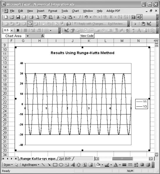
These results look far better than those obtained earlier. Clearly, the results shown in Figure 11-6 for y1 and y3 are sinusoidal as expected. The difference between these results and those obtained using Euler's method are dramatic and effectively illustrate the relative accuracy of higher-order methods, such as the Runge-Kutta method, over Euler's basic method.

Take note of the lines of code Application.ScreenUpdating = False and Application.ScreenUpdating = True at the beginning and end of this subroutine, respectively. These lines turn screen updating off and then back on. This subroutine generates a lot of results, so I turned off screen updating to speed up the calculations. At the end, I turned it back on so the final results are displayed. The line Application.ActiveWorkbook.Save saves the workbook just in case I forget to do so.