Forecasting

Problem

You need to make a forecast of future values given historical values for a time series.

Solution

Excel does not provide built-in functionality for sophisticated forecasting . It does have a FORECAST spreadsheet function that sounds enticing; however, that merely uses a linear trendline and is unsuitable for time series that exhibit significant seasonal variability.

As an alternative, you could use the various moving average techniques to make near-term forecasts. Or you could use some higher-order regression equation (see Chapter 8) to make near-term predictions. Keep in mind that extrapolating too far beyond the extents of the original time series could result in significant errors.

If you have the resources, you could purchase one of the many Excel add-ins that offer sophisticated autoregressive moving average (ARMA) or neural network techniques. If you're so inclined, you can even program such techniques yourself in VBA.

In lieu of all these approaches, you can use standard spreadsheet techniques to make forecasts. I'll show you how by extending the techniques discussed in the previous several recipes.

Discussion

I'll again use the time series shown in Figure 6-23. Recall that this series consists of average monthly temperatures in Louisiana from January 1996 to December 1999. The task now is to make a forecast for the average monthly temperatures in the year 2000.

The brunt of this forecasting effort has already been covered in the previous recipes, in which I showed you how to decompose the time series into its various components using the model Y = TSI. (If you have not read the previous three recipes, you should do so now for relevant background discussion and calculations.)

In Recipe 6.8 I showed you how to compute the long-term trend component, T, for this example time series. Also, in Recipe 6.7 I showed you how to compute the seasonal indices for this example time series.

Now we'll put those results together to make a forecast for the year 2000. We can do so by computing Yf = TS. Here Yf represents the forecast temperature values. T represents the long-term trend, this time extended out over the year 2000. And S represents the seasonal indices as before.

I've ignored the irregular variability component here. This component requires a more sophisticated modeling approach such as an ARMA or neural network approach. As you'll see shortly, we still get fairly good predictions without this component. Further, you could take this irregular variability into account when computing confidence intervals on your predictions by using techniques discussed in Chapter 5.

So all you really need to do now is compute the long-term trend values for the year 2000 using the trend equation from the previous recipe. Then multiply these trend values by the seasonal index for each corresponding month to arrive at a prediction for each month in the year 2000. Figure 6-28 shows a spreadsheet I set up to perform these calculations.

Figure 6-28. Year 2000 forecast

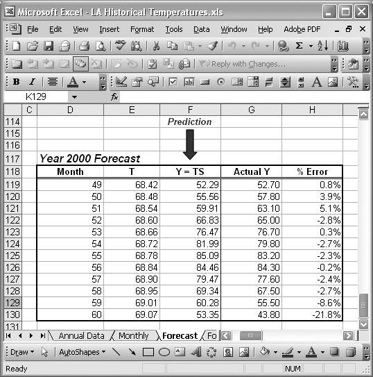
The column labeled Month contains the months representing the year 2000 as an extension of the original series, in which December 1999 was month number 48. You need to number the months for the year 2000 this way because the trendline equation computed in the previous recipe is based on the original monthly series from months 1 to 48 and now we're extending that trend out over another 12 months.

Column T in Figure 6-28 shows the results of the forecast trend in the year 2000. The formulas in this column are of the form =0.0592*D119+65.521.

Column Y = TS contains the predicted average monthly temperatures for the year 2000. These are computed by multiplying each trend value for the year 2000 by the corresponding seasonal index for each corresponding month. For example, the predicted value for January 2000, cell F119, is computed using the formula =E119*Jan. Here again, I'm making use of the cell names I set up corresponding to each seasonal index computed in Recipe 6.7.

Figure 6-29 shows the predicted results compared to the actual average monthly temperatures on record for the year 2000.

Figure 6-29. Year 2000 forecast chart

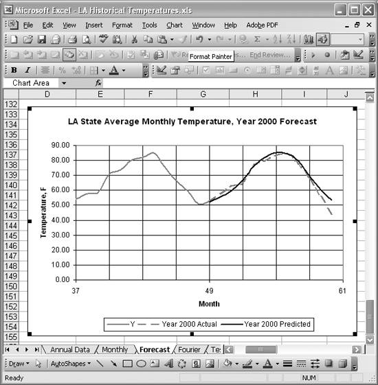
As you can see, these predictions are fairly good. They won't get me a starring role as the local weatherman, but they're not bad for such a simple forecast model. The table in Figure 6-28 also contains computed %Error values, and you can see that errors are on the order of a few percent except for the months of November and December.

The forecasting technique shown in this recipe is by no means the only technique available to you. Time series forecasting is a huge field of study and there are many techniques and models available, many of which are tailored to specific kinds of time series. The examples discussed here serve to show how you can leverage Excel's standard functionality to perform predictions.