Entering Formulas | Using Excel

Problem

You've entered data and are ready to perform some calculations, but don't know how.

Figure 1-9. Group of selected cells

Solution

You need to enter cell formulas in order to perform calculations on data contained in other cells. Entering a formula is simple enough: simply select a cell to hold the formula and then type the equals sign followed by your formula, which can refer to other cells that contain data. A formula to add two numbers contained in cells A1 and A2 would look like this: =A1+A2.

Discussion

All formulas start with an equals sign, as in the =A1+A2 example. You can enter a formula in the same way you enter text, as discussed in Recipe 1.2. You can either enter the formula directly in a cell (pressing Enter when done), or you can use the formula bar, as discussed earlier. The cell containing the formula will display the result of the formula and not the formula itself. To see the formula, just look at the formula bar when the cell is selected. Or press the F2 shortcut key to edit the formula directly in the cell, as shown in Figure 1-10.

Figure 1-10. Entering formulas

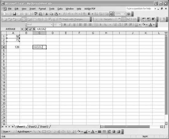
The cell in column C row 4 contains a formula to divide the number contained in column A row 1 by that in column A row 2. I pressed F2 to display the formula for editing directly in the cell.

Formulas may contain the usual mathematical operators such as +, -, /, and *, as well as any number of other built-in functions, as discussed in Recipe 1.10.

I should mention here that spreadsheets are a bit different from procedural programs with which you may be used to working. With a procedural program, you have to explicitly run it after writing the code (we'll do this when we write custom macros and functions using Visual Basic for Applications in Chapter 2). However, once you write a formula in a spreadsheet cell, it executes and remains up-to-date automatically. Therefore, if you change the data in cells referred to by a formula, the results of the formula are updated immediately. Excel takes care of making sure your spreadsheet calculations are updated whenever you change anything.

Excel performs calculations on the stored values of cells (not the displayed values), using 15 digits of precision.

To really leverage formulas, you must understand cell references . In the formula =A1+A2, the data contained in the cells in rows 1 and 2 of column A are referenced as A1 and A2, respectively. In Excel such references are called A1-style references. The letter refers to the column; the number refers to the row number.

References to cells such as A1 are by default relative references . When a relative reference to a cell appears in a formula, that cell is referred to in terms of its relative position to the cell containing the formula. If you cut or copy the formula and then paste it someplace else, the cell references in the formula will automatically change so that they refer to cells in the same relative position to the formula as before. This is better explained by way of example.

In Figure 1-10, the cell A4 contains the formula =A1+A2, which uses relative references. If I copy and paste the formula from cell A4 to cell A5, then the new formula will be =A2+A3. I moved the formula one row down, so the relative cell references were also adjusted by one row. If I moved the formula to column B, then the cell references would have changed from A to B.

This behavior may seem a bit unusual at first, but the advantage of it is clear when you are setting up tables of data and formulas to manipulate the data. For example, say I had two columns of data, B and C, as shown in Figure 1-11.

Figure 1-11. Relative cell references

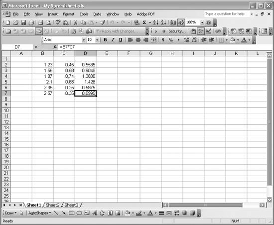
Now in column D, I want to enter a formula to multiply each number in column B by the corresponding number (on the same row) in column C. To do this, I can enter the formula =B2*C2 in cell D2 to yield the product of numbers in cells B2 and C2. For all the remaining rows, I can simply copy and paste the formula in cell D2 into cells from D3 to D7, and Excel will automatically adjust the row numbers in the formulas. For example, after such copying and pasting, cell D7 contains the formula =B7*C7. This saves you the time of having to rewrite each formula directly. Relative cell references are also important when performing certain database filtering operations, as we'll discuss later.

As useful as relative references are, they aren't always want you want. Let's say you have the data as shown in Figure 1-11, but instead of just taking the product of the two numbers in columns B and C, you want to also multiply this product by a single number contained in cell A1. Let's say you want every product shown in column D to be multiplied by that same factor in cell A1. You might enter a formula in cell D2 like =B2*C2*A1. This works for the first result contained in cell D2, but if you copy and paste this formula into cells D3 through D7, the cell reference A1 will also be adjusted by 1 each time, resulting in the formula =(B7*C7)*A6 in cell D7. This isn't want you want, since there are no values in cells A2 through A6. To force Excel to refer to a specific cell you need to use an absolute cell reference. This essentially fixes the cell reference to always refer to a specific cell no matter how the formula is moved or copied. The syntax for an absolute reference to cell A1 in our example looks like =(B2*C2)*$A$1.

The $ symbol in the cell reference indicates to Excel that you want to use absolute references. In this case we fixed both the column and the row in the example cell reference. If we wanted to fix just the column, we would write $A1. Likewise, we could fix just the row by writing A$1.

When entering a formula in a cell, you can select another cell from the spreadsheet to include that cell's reference in the formula. You can also press F4 to cycle through the reference styles for the cell being referred to.

I use absolute references most often when performing calculations on datasets using formulas that refer to common scientific or engineering constants.

Formulas cannot refer to themselves. For example, if you put a formula in cell A3, it cannot contain a reference to cell A3. That's called a circular reference, and Excel will give you a warning message if one occurs.