Constructing Your Own Linear Fit Using Spreadsheet Functions

Problem

You want to perform a linear curve fit using standard least-squares formulas instead of Excel's linear trendline.

Solution

Use Excel's built-in formulas such as COUNT, SUM, SUMSQ, and SUMPRODUCT to make it easy to apply the standard least-squares formulas.

Discussion

The standard equation for a straight line is:

The standard least-squares formulas used to determine the slope, m, and intercept, b, of the fit line are:

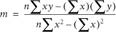
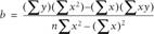
In these equations, n is the number of data points. Excel has several built-in functions that make it very easy to compute the various sums that appear in the least-squares equations. These functions include:

COUNT

This function counts the number of cells containing numbers in a range of cells.

SUM

This function adds all the numbers in a range of cells.

SUMSQ

This function returns the sum of squares of the numbers contained in a range of cells.

SUMPRODUCT

This function sums the products of entries in corresponding ranges of cells.

Let's reconsider the data used in the example in Recipe 8.1. Instead of using a chart trendline to determine the best-fit line, we'll use the least-squares equations and built-in Excel functions. Figure 8-4 shows a simple spreadsheet I set up for this example.

The columns labeled X and Y contain the same data as before. I just renamed them to make it easier to follow the application of the formulas used in this example. Cells B23 through B27 contain formulas to compute the various quantities required by the least-squares formula. The formulas in these cells are as follows:

Cell B23

The formula in this cell, =COUNT(A4:A21), computes the number of data points.

Cell B24

The formula in this cell, =SUM(A4:A21), computes the sum of x-values.

Cell B25

The formula in this cell, =SUM(B4:B21), computes the sum of y-values.

Cell B26

The formula in this cell, =SUMPRODUCT(A4:A21,B4:B21), computes the sum of the products on values in the X and Y columns.

Cell B27

The formula in this cell, =SUMSQ(A4:A21), computes the sum of squares of x-values.

Figure 8-4. Least-squares fit

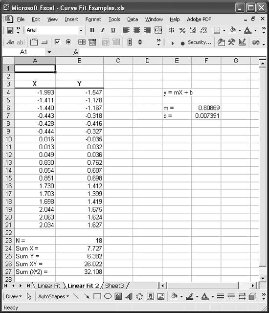
These cells contain all of the data we need to apply the least-squares formulas.

Cell F6 computes the slope of the best-fit line. The formula in cell F6 is =(B23*B26-B24*B25)/(B23*B27-B24^2). The formula in cell F7, =(B25*B27-B24*B26)/(B23*B27-B24^2), computes the y-intercept for the best-fit line.

The resulting slope and intercept are 0.80869 and 0.007391, respectively. These values agree very well with those obtained using a trendline as discussed in Recipe 8.1.

To assess how well this fit equation represents the data, you can compute the R-squared value just as Excel does when it computes chart trendlines. The closer R-squared is to 1, the better the fit. Read Recipe 8.7 to learn more about the R-squared value.

For this example, you need to perform a few more calculations in order to compute the R-squared value. Namely, you need to compute the mean of the y-values, the estimated y-values, and the residuals. Figure 8-5 shows these new calculations for this example. Cell F10 computes the mean y-value using Excel's AVERAGE function. Column H contains the estimated y-values using the equation for a straight line, along with the computed slope and intercept. Columns I and J are used to calculate the differences between the estimated y-values and the mean and between the actual y-values and the mean, respectively. The sums of the squares of these differences are computed in cells I22 and J22 using Excel's SUMSQ function.

Figure 8-5. R-squared computation

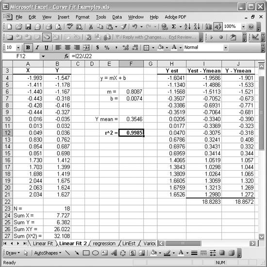
The R-squared value is computed in cell F12 by simply taking the ratio of the values in cells I22 and J22. In Figure 8-5, cell F12 is selected and you can see the cell formula for computing R-squared in the formula bar. For this example, R-squared comes out to 0.9985, which indicates a good fit and agrees very well with the value obtained using a chart trendline as discussed in Recipe 8.1.