Integrating a Definite Integral | Numerical Integration and Differentiation

Problem

You have an analytic function that you need to integrate numerically.

Solution

Use the trapezoidal rule of numerical integration.

Discussion

As discussed in the introduction to this chapter, there exists a multitude of numerical integration formulas and rules to choose from. Your choice depends on several factors including, but not limited to, desired accuracy and ease of implementation. For the purposes of this example, I want to use one of the easiest to implement numerical integration rules, namely the trapezoidal rule. This rule exemplifies the main steps in setting up numerical integration in a spreadsheet without clouding the issue with more complicated mathematics.

In this example, I'll consider the integration of a given analytic function of the form:

where the analytic form of f(x) is known. Even though you know f(x), you may not be able to integrate it analytically, and this is one reason why you would resort to numerical integration.

The trapezoidal rule is well documented in virtually every calculus, engineering analysis, or numerical methods book I've ever read. Basically, this technique approximates the function under consideration with a sequence of linear curves. The general formula (also called extended or composite formula) for the trapezoidal rule is:

Here, s is the distance along the x-axis between samples. This formula assumes that all of the y-values are computed, or correspond, to equally spaced x-values. Since we have an analytic form of f(x), we can easily choose the spacing and thus the number of x-values between the bounds of integration a and b. The smaller the spacing and the greater the number of samples, the higher the accuracy.

Excel is very well suited to integration formulas like the trapezoidal rule. In fact, many popular integration rules are of similar form, in that they consist of the sum of products between coefficients and y-values. This sort of computation is easily set up in Excel.

Figure 10-1 shows a spreadsheet that uses the trapezoidal rule to compute the integral of the function:

for x in the interval [0,1].

Figure 10-1. Trapezoidal rule example

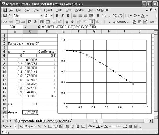
The first step in performing this integration is to set up a table containing the x-values and corresponding y-values. I selected a spacing of 0.1 between x-values and put them in column B. The y-values are computed in column C using formulas like =EXP(-(B6^2)).

The next step is to set up a column containing the coefficients that appear in the integration formula. This is almost trivial in the case of the trapezoidal rule, since all but the first and last coefficients are 1, but it's a very handy way to organize the coefficients for other rules that don't involve a bunch of ones.

I put the x-spacing value (s = 0.1) in cell C18, just for clarity. Cell C20 contains the actual trapezoidal rule formula. This cell is selected in the screenshot so you can see the formula in the formula bar toward the top of the spreadsheet. The formula is =C18*SUMPRODUCT(C6:C16,D6:D16) and it uses the SUMPRODUCT worksheet function to compute the sum of the products of the y-values and the coefficients. The result in this case is 0.746 and represents the area under the curve from x = 0 to x = 1.

In many cases, you won't necessarily have an analytic function with which to work. You may be dealing with experimental data or functions represented by tabular values. You can apply the technique discussed in this recipe in just the same way. Instead of evaluating the given function to populate a y-column as shown in Figure 10-1, you would simply use your sampled or tabulated y-data. The rest of the calculation is the same as discussed here. See Recipes 10.3 and 10.4 for some examples using tabulated data.

The trapezoidal rule shown here is very easy to implement, which makes it very attractive. The theoretical error of the trapezoidal rule is proportional to spacing between samples to the third power. If you increase the number of samples so as to decrease the spacing by a factor of 2, then the error will decrease by a factor of 8. Looking at this from another angle, for the example discussed here, reducing the spacing by a factor of 2 from 0.1 to 0.05 only affects the result beyond the fourth digit after the decimal place. The result goes from 0.746211 to 0.746671.

Increasing the number of samples (thus decreasing the spacing) is one way to improve accuracy when using the trapezoidal rule. Some practitioners take an iterative approach and stop increasing the number of samples when changes in the result from successive iterations fall below some tolerance (see Recipe 10.2).

There are other ways to improve the accuracy of numerical integration. An obvious way is to use a rule or method that is inherently more accurate. One very well-known rule is called Gaussian quadrature or Gaussian integration.

There are many other, inherently more accurate rules, many of which are easier to implement than Gaussian quadrature and which are better suited for tabulated data in lieu of having a known analytic function. Recipes 10.3 and 10.4 discuss examples using Simpson's rule for tabulated data, which is just as easy to implement as the trapezoidal rule, and more accurate.

For now, let's consider the same problem discussed earlier but this time solved using Gaussian integration. The idea behind Gaussian integration is that an integral of a function over a standard interval can be approximated by the weighted sum of functional values over that interval. In equation form this looks like:

There are a couple of tricks to applying this method. First, for integrals over nonstandard intervals, you have to transform (usually using a linear transformation) the actual interval to the standard interval, using a change of variables. Also, you need to derive the proper coefficients by which to multiply the functional values over the interval.

Fortunately, there are several different standard Gaussian integration formulas that have already been derived and are readily available from standard texts on the subject of numerical methods. Once such standard formula is the fifth-order formula :

To apply this formula to the example function discussed in this recipe, the first thing you need to do is transform from variable x over the interval from 0 to 1 to a variable t over the interval from -1 to 1. To do this, let t = 2x - 1. Then x = (t + 1)/2, which gives dx = (1/2)dt. Now we have:

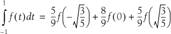
And the integral to be evaluated is now:

The 1/2 factor comes from the change of variables dx = (1/2)dt. Applying the Gaussian formula in a spreadsheet cell formula looks like this:

 =0.5 * (5/9 * f_of_t(-SQRT(3/5)) + 8/9 * f_of_t(0) + 5/9 * f_of_t(SQRT(3/5)))

This formula uses a custom VBA function named f_of_t, which simply evaluates the function f(t) shown earlier. The VBA code for this function is shown in Example 10-1.

Example 10-1. VBA code for f_of_t

Public Function f_of_t(t As Double) As Double
 f_of_t = Exp(-(1 / 4#) * (t + 1) ^ 2)
End Function

You don't have to use a custom VBA function as I did here. I did so only to make the spreadsheet formula more readable.

The end result for this example is 0.746814. Comparing this result to that obtained using the trapezoidal rule shows that the results are identical out to the third decimal place. To make the result from the trapezoidal rule equal that obtained from the Gaussian formula out to the fourth decimal place, you'd have to increase the number of samples to 53. To make the result identical to the fifth decimal place, you'd have to increase the number of samples to 67. (I obtained these values iteratively.)

There are two ways to view these results. On one hand, it's clear that the required number of samples when using the trapezoidal rule is higher for the same level of accuracy. On the other hand, in this example at least, the higher number of samples results in an insignificant increase in computational time, whereas applying the Gaussian formula is certainly more effort.

I have to be honest here. I've never applied the Gaussian formula to solve any real-world problem. I've always found it too easy to simply increase the number of samples when using the trapezoidal rule, or more often Simpson's rule, and live with the few extra milliseconds it takes to compute the result, given the power of modern desktop computers. This works for me, but it's not to say the same will work for the type of problems that require you to implement numerical integration.