Fitting Nonlinear Curves Using Solver

Problem

You'd like to perform a curve fit using a model (an equation) that's not included in Excel's suite of curve fit functions and trendlines.

Solution

Perform a least-squares curve fit using Solver.

Discussion

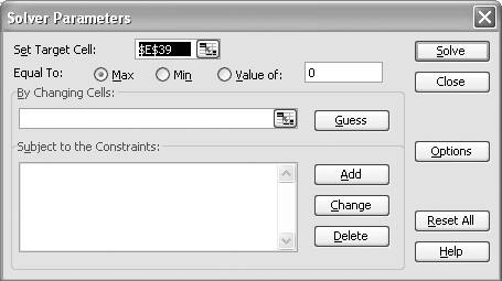
Solver is a fantastic Excel add-in that allows you to perform constrained optimization calculations. Solver uses the nonlinear Generalized Reduced Gradient optimization algorithm developed by Leon Lasdon and Allan Waren. Go to the Tools images/U2192.jpg border=0> Solver menu to open the Solver dialog box shown in Figure 8-10.

Figure 8-10. Solver dialog box

If you don't see the Solver menu item, then go to Tools images/U2192.jpg border=0> Add-Ins...and look for Solver in the available add-ins list. Select its checkbox to make it available.

Solver allows you to choose a target cell and either maximize it, minimize it, or attempt to set its value to some specified value by changing values in a given range of cells. The controls in the Solver dialog box allow you to set these parameters. After setting these parameters in the Solver dialog box, press Solve to initiate the iterative calculation. Solver will iterate until it finds a solution or until certain limits are reached (these effectively put the brakes on the iterative calculation so it will not continue forever). You can set these limits by opening the Options dialog via the Options button.

The target cell could be any cell containing a formula. That formula could contain references to other cells, which could themselves contain formulas, and so on. Ultimately, the value in the target cell will be affected by certain parameters contained in a select group of cells or a single cell. You can construct arbitrarily complex spreadsheets that somehow relate the target cell to one or more cells containing values, such as constants or coefficients. This is really powerful. You can create spreadsheets to compute something subject to a given set of inputs and then you can use Solver to find the optimum set of inputs to maximize, minimize, or specify the output. It's this facility that we'll leverage to use Solver for nonlinear curve fitting.

Ultimately, curve fitting involves minimizing some error, which can be expressed as the sum of squared differences between actual and predicted values as in the least-squares method. You could use some other merit function instead of the sum of squared residuals. For example, you could choose to maximize the coefficient of determination, R-squared, instead.

The basic approach to using Solver for curve fitting is to set up a spreadsheet containing sample data for your dependent and independent variables. The dependent variable will be predicted using some model (i.e., an equation) that you devise. Set up another column for predictions of your dependent variable using your model equation. Add another column containing the residuals (i.e., the differences between your predicted value and the actual value of the dependent variable). Compute the sum of squared differences in another cell. In the case of minimizing the sum of squared differences, you can set this cell as the target cell in the Solver dialog box. Set the option to minimize that cell. Your model equation must contain parameters, or coefficients. These should be located conveniently in another set of cells. Use references to these cells as the cells to change in the Solver dialog box. Solver will then attempt to minimize the sum of squared differences with the end result, if it succeeds, being the set of parameters that yield the optimum solution. This gives you the curve fit.

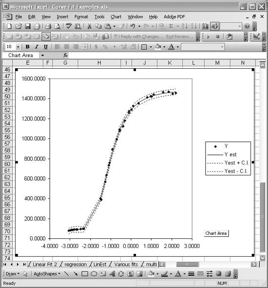
Let's look at an example. We'll consider a standard reference set of data available from the NIST web site. In this case, the data is from an NIST study involving semi-conductor electron mobility where the dependent variable, y, is a measure of electron mobility, and the independent variable, x, is the natural log of the density.[*] The model for this data is nonlinear and of the following form:

[*] This dataset is credited to R. Thurber of NIST and is available for download from http://www.nist.gov.

The bs in this equation are the parameters to be determined through the fitting processes. There are seven of them. Clearly, this nonlinear, rational function is not included in Excel's suite of curve-fitting tools. This illustrates the generality of using Solver for curve fittingyou can use any model equation you want.

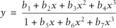
Figure 8-11 shows a portion of the data used for this example. There are 37 data points contained in columns D and E. As you can see, I set up a little table of b-coefficients off to the left. These are set up with some initial values that you must choose. These cells don't contain formulas. Just type the numbers in directly; Solver will change them during its calculations.

Figure 8-11. Example data

You have to provide an initial guess at the model parameters, the bs in this example. This is the case with many iterative algorithms. You must choose these wisely given the problem you are considering and in light of your understanding of it. It's best to make as good an educated guess as possible. If your model is highly nonlinear, there may be several solutions. As with nonlinear optimization problems in general, there could exist local minima and maxima in the merit function domain within which Solver may converge on a solution. I recommend you try several different sets of initial values to make sure you're converging on a global optimum as opposed to some local optimum.

Column G contains the estimated y-value for each x-value in the dataset. This estimated y-value uses the model equation. In this case, I coded the model equation in a custom VBA function called CalcYest (see Recipe 2.2). CalcYest is shown in Example 8-1.

Example 8-1. CalcYest

Function CalcYest(x As Double, b1 As Double, b2 As Double, b3 As Double,
 b4 As Double, b5 As Double, b6 As Double,
 b7 As Double) As Double

 CalcYest = (b1 + b2 * x + b3 * x ^ 2 + b4 * x ^ 3) /
 (1 + b5 * x + b6 * x ^ 2 + b7 * x ^ 3)

End Function

This function takes the x-value along with all seven b-parameters as arguments and returns the estimated y-value. You'll notice in Figure 8-11 that cell G5 is selected. Take a look at the formula bar to see how CalcYest is actually used as a cell formula.

The table off to the right in Figure 8-11 contains several statistics that I computed for this example. I'll address most of these later (see Recipes 8.7 and 8.8), so for now just look at cell M5. That cell contains the sum of squared residuals. The residuals are computed in column H and are simply the estimated y-values minus the sampled y-values. The sum of squared residuals is computed in cell M5 with the formula =SUMSQ(H5:H41). SUMSQ is Excel's built-in function that computes the sum of the squares of the values contained in the given range. It's this value we want to minimize for the curve fit.

With things set up as described, you can now open Solver and set the parameters. First set the target cell to M5, the sum of squared residuals. Next select the "Equal to: Min" option, letting Solver know we want to minimize the value contained in M5. Enter the cell range B4:B10 in the By Changing Cells field. Press the Solve button. At this point, another dialog box will open, showing the results of Solver's calculations. Solver will tell you whether or not it converged on a solution and will give you the option of saving its results or restoring your original values (the values of the parameters you allowed Solver to change).

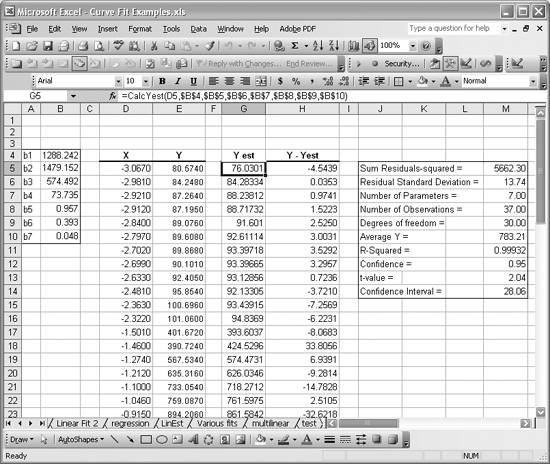
The converged results for this example are already shown in Figure 8-11. The b-parameters computed here agree very well with the NIST benchmark results. Further, the R-squared value for this example is 0.99932, indicating a good fit. Figure 8-12 shows the results plotted on a chart along with the original data. The original data points are shown with diamond point markers, and the estimated values are shown with the solid curve. The two other curves above and below the estimate curve represent the 95% confidence interval for the predicted values. See Recipe 8.8 to learn how to compute these curves.

Figure 8-12. Solver curve-fit results

Clearly, this approach using Solver yields a nice curve fit to a fairly nonlinear set of data. I must say that not all nonlinear curve fits are this straightforward. I've had some very unruly cases involving multiple nonlinear models, where a different local minimum was converged upon for virtually every set of guessed input parameters I could imagine. In other cases, the model was such that Solver could not converge on a solution at all. These aren't necessarily a defect in this approach or a deficiency in Solver. Those of you who've experienced such difficulties firsthand know that it's just the nature of some highly nonlinear problems to make your life difficult.