Optimizing The Oracle Side

Any query that returns data and runs against Oracle goes through three general steps. First, the query is parsed and an execution plan is determined, then it is executed, and finally the caller fetches the results. This chapter describes Oracle optimizers and execution plans. Optimizer hints useful to a report writer are described, and effective indexing strategies are covered. The use of stored outlines is also explained. A subreport will be developed that shows the execution plan for a report query.

Material in this chapter should not be considered an exhaustive description of the related Oracle processes. Please refer to Oracle documentation for complete coverage.

Oracle Optimizers

A general knowledge of the Oracle optimizers is required in order to understand execution plan optimization. Though the argument could be made that optimization is the domain of the DBA only, it would be shortsighted. The report developer can contribute much toward the creation of reusable, resource-efficient, optimized queries. The DBA’s outlook is the entire system; the report developer can concentrate on a much smaller portion of that system, namely the report query.

Oracle has two optimizers, the older rule-based optimizer, and the newer cost-based optimizer. These optimizers are responsible for generating an execution plan for each query. The execution plan is a set of steps that the DBMS will follow to get the data required by the query. The default optimizer for the instance is set using the OPTIMIZER_MODE initialization parameter. The default value for OPTIMIZER_MODE for Oracle 8i and Oracle 9i is CHOOSE. The instance’s optimizer mode can be overridden for a session by using ALTER SESSION, or for a particular query by using optimizer hints in the statement.

Rule Based

The rule-based optimizer makes decisions about the optimal execution plan for a given query based on a set of rules. A full discussion of these rules is outside the scope of this book, but the type of information that is stored in the database dictionary drives them. The rules are based on information about table definitions, index definitions, clustering, and so on in combination with the requirements of the query. No matter what data is stored in the database, the rule-based optimizer will always make the same decision. The rule-based optimizer will be used if the OPTIMIZER_MODE is set to RULE, or if no database statistics are available.

Cost Based

The cost-based optimizer uses database statistics such as the number of rows in a table and the key spread, in combination with object definitions, to determine the optimal execution plan. The cost-based optimizer will calculate a cost for each possible execution plan and choose the least costly. In order to function, the cost-based optimizer requires that database statistics are available. The cost-based optimizer will be used if the OPTIMIZER_MODE is set to CHOOSE and at least one table in the query has statistics calculated for it. For the CHOOSE optimizer mode, the cost-based optimizer will choose the best execution plan that returns all rows. If the optimizer mode is set to FIRST_ROWS_n or ALL_ROWS, the cost-based optimizer will be used whether or not statistics exist. ALL_ROWS will optimize for total throughput, whereas FIRST_ROWS_n will optimize for the speediest return of the first n rows, where n can be 1, 10, 100, or 1000. The FIRST_ROWS optimizer mode exists for backward compatibility.

Gathering Statistics

Gathering database statistics is the domain of the DBA, and there are multiple methods in which to do this. Shown next is Oracle 9i sample code for gathering statistics for the XTREME schema that uses the DBMS_STATS package. A report developer would not usually be gathering statistics. This topic is mentioned for two reasons. One, if you see unexpected results when viewing execution plans, you will have the background to realize that statistics may be stale. Two, this script should be run so that the examples later in the book will work. Statistics should be gathered regularly so that the cost-based optimizer can make valid decisions.

BEGIN
DBMS_STATS.GATHER_SCHEMA_STATS(
 OWNNAME=>'XTREME',
 ESTIMATE_PERCENT=>DBMS_STATS.AUTO_SAMPLE_SIZE,
 CASCADE=>TRUE,
 OPTIONS=>'GATHER AUTO',
 METHOD_OPT=>'FOR ALL INDEXED COLUMNS');
-- Skewed column ORDERS.SHIPPED
DBMS_STATS.GATHER_TABLE_STATS(
 OWNNAME=>'XTREME', TABNAME=>'ORDERS',
 ESTIMATE_PERCENT=>DBMS_STATS.AUTO_SAMPLE_SIZE,
 CASCADE=>TRUE,
 METHOD_OPT=>'FOR COLUMNS SIZE AUTO SHIPPED');
END;

Here is a script for Oracle 8i:

BEGIN
DBMS_STATS.GATHER_SCHEMA_STATS(
 OWNNAME=>'XTREME',
 CASCADE=>TRUE,
 OPTIONS=>'GATHER',
 METHOD_OPT=>'FOR ALL INDEXED COLUMNS');
-- Skewed column ORDERS.SHIPPED
DBMS_STATS.GATHER_TABLE_STATS(
 OWNNAME=>'XTREME', TABNAME=>'ORDERS', 
 CASCADE=>TRUE,
 METHOD_OPT=>'FOR COLUMNS SIZE 100 SHIPPED');
END;

Execution Plans

An execution plan is the systematic process that Oracle will go through to retrieve the data required to satisfy the query. For a query backing a report, data retrieval will usually be the most time-consuming and resource-intensive portion of the process. The parser checks the syntax and verifies the existence of objects and may rewrite queries containing views, subqueries, or IN clauses. It may also convert a query to use an existing materialized view instead of base tables. The parser then determines an optimal access path, from which it produces an execution plan.

The optimizer goal as shown in an execution plan can be CHOOSE or RULE. If the COST field is populated, the cost-based optimizer was used. If it is null, the rule-based optimizer was used.

Displaying Execution Plans

Execution plans can be displayed using the Explain Plan directive in SQL*Plus, Oracle trace files, or they can be queried from the dynamic performance views. The “Execution Plan Subreport” section later in this chapter shows how to use a Crystal subreport to display the actual execution plan used in the report. In this section, Explain Plan will be used to demonstrate what execution plans look like. To use Explain Plan, you must have access to a PLAN_TABLE. The SQL script UTLXPLAN.SQL, usually found in the Oracle_HomeRDBMSAdmin directory and included in the download files for this chapter, creates the PLAN_TABLE. The PLAN_TABLE for the XTREME schema was created in Chapter 1 with the other schema objects.

To populate the PLAN_TABLE, run a statement of the following form from a SQL*Plus prompt:

EXPLAIN PLAN FOR <>

See Oracle documentation for a full description of the EXPLAIN PLAN statement. The plan can be put into a table other than the PLAN_TABLE or identified with a statement_id using other available options.

To display the execution plan, you can use a supplied PL/SQL package (9i), a supplied database script, or you can query the PLAN_TABLE directly as shown:

SELECT id, cardinality "Rows",
 SUBSTR(lpad(' ',level-1)
 ||operation||' '||options||' '||object_name, 1, 40) Plan, 
 SUBSTR(optimizer,1,10) Optimizer, cost, bytes 
 FROM PLAN_TABLE
WHERE timestamp=(SELECT MAX(timestamp) FROM plan_table)
CONNECT BY prior id = parent_id
 AND prior timestamp = timestamp
 START WITH id = 0
ORDER BY id;

To use the PL/SQL package for 9i, run the following:

SELECT plan_table_output 
 FROM TABLE(DBMS_XPLAN.DISPLAY('plan_table',null,'all'));

See Figure 7-1 for a complete example. See Oracle documentation for a full description of the DBMS_XPLAN package.

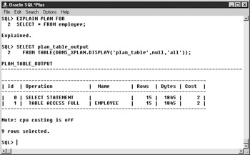
Figure 7-1: DBMS_XPLAN example

To use the supplied SQL scripts, run UTLXPLS.SQL for nonpartitioned queries or UTLXPLP.SQL for partitioned queries. These scripts can be found in the Oracle_HomeRDBMSAdmin directory or in the download files for this chapter.

The order of steps in the execution plan in the display is not the order in which those steps are actually executed. The execution starts at the leaf nodes and works up from there. The predicate information section shows the actual joining and filtering conditions from the query.

Access Methods

The execution plan will tell you what table access methods will be used. There are several possible methods of table access, including full table scan, index lookup, and ROWID.

Full Table Scan

A full table scan means that the entire table is read up to the high water mark, which is the last block that had data written to it. If a table is highly unstable, it should be reorganized frequently to ensure that the high water mark is conservative. Full table scans use multiblock IO, and how many blocks are read is determined by the system parameter DB_FILE_MULTIBLOCK_READ_COUNT. Blocks read in a full table scan are placed at the least recently used end of the buffer cache and will be aged out of the cache quickly. Figure 7-1 shows an execution plan with a full table scan.

Index Lookup

Index lookup uses an index to look up the necessary ROWIDs and then reads the rows from the table using the ROWID. Index lookups use single block IO. If all of the required columns are in the index, no table access will be performed. If the ORDER BY clause of the query matches the index used, no sort will be required.

Note

All the following examples use Oracle 9i. 8i results would be similar.

Index Unique Scan

The Index unique scan looks up a single index value. All columns of the index must be used in the WHERE clause of the query with equality operators.

SQL> EXPLAIN PLAN FOR
 2 SELECT * FROM employee
 3 WHERE employee_id=5;


Explained.


SQL> SELECT plan_table_output 
 2 FROM TABLE(DBMS_XPLAN.DISPLAY('plan_table',null,'all'));


PLAN_TABLE_OUTPUT
---------------------------------------------------------------------
| Id | Operation | Name |Rows |Bytes|Cost|
---------------------------------------------------------------------
| 0 | SELECT STATEMENT | | 1| 123| 1 |
| 1 | TABLE ACCESS BY INDEX ROWID| EMPLOYEE | 1| 123| 1 |
|* 2 | INDEX UNIQUE SCAN | EMPLOYEE_PK | 15| | |
---------------------------------------------------------------------
Predicate Information (identified by operation id): 
---------------------------------------------------
 2 - access("EMPLOYEE"."EMPLOYEE_ID"=5) 


Note: cpu costing is off

Index Range Scan

The index range scan method looks up a range of key values. One or more of the leading columns of the index must be used in the query. Rows are returned in index order.

SQL> EXPLAIN PLAN FOR
 2 SELECT * FROM orders
 3 WHERE order_id > 3150;


Explained.


SQL> SELECT plan_table_output
 2 FROM TABLE(DBMS_XPLAN.DISPLAY('plan_table',null,'all'));


PLAN_TABLE_OUTPUT
---------------------------------------------------------------------
| Id | Operation | Name | Rows |Bytes|Cost|
---------------------------------------------------------------------
| 0 | SELECT STATEMENT | | 30| 2310| 3|
| 1 | TABLE ACCESS BY INDEX ROWID| ORDERS | 30| 2310| 3|
|* 2 | INDEX RANGE SCAN | ORDERS_PK | 30| | 2|
----------------------------------------------------------------------
Predicate Information (identified by operation id):
---------------------------------------------------
 2 - access("ORDERS"."ORDER_ID">3150)


Note: cpu costing is off

Index Range Scan Descending

Index range scan descending is used when an ORDER BY DESC clause that can use an index is in the query; it is identical to an index range scan except that data is returned in descending index order.

SQL> EXPLAIN PLAN FOR
 2 SELECT * FROM orders
 3 WHERE order_id > 3150
 4 ORDER BY order_id DESC;


Explained.


SQL> SELECT plan_table_output
 2 FROM TABLE(DBMS_XPLAN.DISPLAY('plan_table',null,'all'));


PLAN_TABLE_OUTPUT
---------------------------------------------------------------------
| Id | Operation | Name | Rows|Bytes|Cost|
---------------------------------------------------------------------
| 0 | SELECT STATEMENT | | 30| 2310| 3|
| 1 | TABLE ACCESS BY INDEX ROWID | ORDERS | 30| 2310| 3|
|* 2 | INDEX RANGE SCAN DESCENDING| ORDERS_PK | 30| | 2|
---------------------------------------------------------------------
Predicate Information (identified by operation id):
---------------------------------------------------
 2 - access("ORDERS"."ORDER_ID">3150)
 filter("ORDERS"."ORDER_ID">3150)


Note: cpu costing is off

Index Skip Scans

Index skip scanning allows indexes to be searched even when the leading columns are not used. This can be faster than scanning the table itself. In the following example, the index ORDERS_SHIPPED_DATE is on columns SHIPPED and SHIP_DATE. SHIPPED, which is the first field in the index, is not used in the query, so the index is skip scanned.

Note

Skip scanning is a new feature of Oracle 9i.

SQL> EXPLAIN PLAN FOR
 2 SELECT * FROM orders
 3 WHERE ship_date=To_DATE('01/12/2000','mm/dd/yyyy');


Explained.


SQL> SELECT plan_table_output
 2 FROM TABLE(DBMS_XPLAN.DISPLAY('plan_table',null,'all'));


PLAN_TABLE_OUTPUT
---------------------------------------------------------------------
|Id|Operation | Name |Rows|Bytes|Cost|
---------------------------------------------------------------------
| 0|SELECT STATEMENT | | 3 | 231 | 5 |
| 1| TABLE ACCESS BY INDEX ROWID|ORDERS | 3 | 231 | 5 |
|*2| INDEX SKIP SCAN |ORDERS_SHIPPED_DATE| 1 | | 3 |
---------------------------------------------------------------------
Predicate Information (identified by operation id):
---------------------------------------------------
 2 - access("ORDERS"."SHIP_DATE"=TO_DATE('2000-01-12 00:00:00',
 'yyyy-mm-dd hh24:mi:ss'))
 filter("ORDERS"."SHIP_DATE"=TO_DATE('2000-01-12 00:00:00',
 'yyyy-mm-dd hh24:mi:ss'))


Note: cpu costing is off

Index Full Scan

Index full scanning reads the entire index in order. It might be used instead of a full table scan if the rows need to be returned in index order, but it uses single block IO and can be inefficient.

Index Fast Full Scan

Index fast full scanning reads the entire index but not in order. It is used only by the cost-based optimizer and uses multiblock IO. It can be used for parallel execution and when the first column of the index is not needed in the query. In the following example, the query returns only the SHIP_DATE column, so even though SHIP_DATE is the second field in the ORDERS_SHIPPED_DATE index, it is faster to read the index than it would be to read the entire ORDERS table.

SQL> EXPLAIN PLAN FOR
 2 SELECT DISTINCT ship_date FROM orders;


Explained.


SQL> SELECT plan_table_output
 2 FROM TABLE(DBMS_XPLAN.DISPLAY('plan_table',null,'all'));


PLAN_TABLE_OUTPUT
---------------------------------------------------------------------
| Id | Operation | Name |Rows|Bytes|Cost|
---------------------------------------------------------------------
| 0 | SELECT STATEMENT | | 731| 5848| 10|
| 1 | SORT UNIQUE | | 731| 5848| 10|
| 2 | INDEX FAST FULL SCAN| ORDERS_SHIPPED_DATE |2192|17536| 4|
---------------------------------------------------------------------


Note: cpu costing is off

ROWID

Using this method, the block with the specified ROWID is read. This is the fastest access method, although it is rare that a query is written explicitly to use a ROWID. This method is most commonly used implicitly with an index lookup. See the index unique scan example in the preceding section.

Joins

The join order is very important in determining an optimal execution plan. If there are more than two tables in a query, the joins will happen in a particular order. First, the first table and the second table will be joined and any filtering conditions that apply to them will be made. Then the third table will be joined to the result of the first join, and so on. The fewer records returned by the first join, the fewer records any subsequent joins have to deal with. The optimizer will determine a join order, but this may be overridden with the ORDERED optimizer hint.

There are three types of joins: the sort merge join, the nested loops join, and the hash join. In addition to the normal join types, a Cartesian product can also be returned.

Sort Merge Join

When two tables are joined using a sort merge join, each table is independently sorted if it is not already sorted on the join fields, and then the two sorted datasets are merged. An Explain Plan includes table access statements and then a merge join statement. Due to the required sorting, this is not an efficient join method.

SQL> EXPLAIN PLAN FOR
 2 SELECT order_id, SUM(order_amount),
 3 SUM(unit_price*quantity) test_amount
 4 FROM orders JOIN orders_detail USING (order_id)
 5 WHERE order_id>3150
 6 GROUP BY order_id;


Explained.


SQL> SELECT plan_table_output
 2 FROM TABLE(DBMS_XPLAN.DISPLAY('plan_table',null,'all'));


PLAN_TABLE_OUTPUT
|Id|Operation | Name |Rows|Bytes|Ct|
---------------------------------------------------------------------
| 0|SELECT STATEMENT | |29| 609|8|
| 1| SORT GROUP BY NOSORT | |29| 609|8|
| 2| MERGE JOIN | |29| 609|8|
| 3| TABLE ACCESS |ORDERS |30| 270|3|
 BY INDEX ROWID
|*4| INDEX RANGE SCAN |ORDERS_PK |30| |2|
|*5| SORT JOIN | |50| 600|5|
| 6| TABLE ACCESS |ORDERS_DETAIL |50| 600|3|
 BY INDEX ROWID
|*7| INDEX RANGE SCAN |ORDERS_DETAIL_ORDER_ID_INDEX| 1| |2|
---------------------------------------------------------------------
Predicate Information (identified by operation id):
---------------------------------------------------
 4 - access("ORDERS"."ORDER_ID">3150)
 5 - access("ORDERS"."ORDER_ID"="ORDERS_DETAIL"."ORDER_ID")
 filter("ORDERS"."ORDER_ID"="ORDERS_DETAIL"."ORDER_ID")
 7 - access("ORDERS_DETAIL"."ORDER_ID">3150)


Note: cpu costing is off

Nested Loops

In nested loop joins, the rows meeting the filtering criteria for the first table are returned. Then, for each row in that result, table two is probed for the matching rows. The number of rows returned by the first table and the speed of access to the second table determines the efficiency of nested loops.

SQL> EXPLAIN PLAN FOR
 2 SELECT order_id, SUM(order_amount),
 3 SUM(unit_price*quantity) test_amount
 4 FROM orders JOIN orders_detail USING (order_id)
 5 WHERE order_id=3150
 5 GROUP BY order_id;


Explained.


SQL> SELECT plan_table_output
 2 FROM TABLE(DBMS_XPLAN.DISPLAY('plan_table',null,'all'));


PLAN_TABLE_OUTPUT
---------------------------------------------------------------------
|Id|Operation | Name |Rows|Bytes|Cst|
---------------------------------------------------------------------
| 0|SELECT STATEMENT | | 1| 21| 4|
| 1| SORT GROUP BY NOSORT | | 1| 21| 4|
| 2| NESTED LOOPS | | 2| 42| 4|
| 3| TABLE ACCESS |ORDERS | 1| 9| 2|
 BY INDEX ROWID
|*4| INDEX UNIQUE SCAN |ORDERS_PK |2192| | 1|
| 5| TABLE ACCESS |ORDERS_DETAIL | 2| 24| 2|
 BY INDEX ROWID
|*6| INDEX RANGE SCAN |ORDERS_DETAIL_ORDER_ID_INDEX| 2| | 1|
---------------------------------------------------------------------
Predicate Information (identified by operation id):
---------------------------------------------------
 4 - access("ORDERS"."ORDER_ID"=3150)
 6 - access("ORDERS_DETAIL"."ORDER_ID"=3150)
Note: cpu costing is off

Hash Join

Only the cost-based optimizer uses hash joins. The data source with the fewest rows is determined, and a hash table and a bitmap are created. The second table is then hashed and matches are looked for.

SQL> EXPLAIN PLAN FOR
 2 SELECT employee_id, first_name, last_name
 3 city, country
 4 FROM employee JOIN employee_addresses USING (employee_id);


Explained.


SQL> SELECT plan_table_output
 2 FROM TABLE(DBMS_XPLAN.DISPLAY('plan_table',null,'all'));


PLAN_TABLE_OUTPUT
--------------------------------------------------------------------
| Id | Operation | Name |Rows|Bytes|Cost|
--------------------------------------------------------------------
| 0 | SELECT STATEMENT | | 15| 405| 5|
|* 1 | HASH JOIN | | 15| 405| 5|
| 2 | TABLE ACCESS FULL | EMPLOYEE | 15| 270| 2|
| 3 | TABLE ACCESS FULL | EMPLOYEE_ADDRESSES | 15| 135| 2|
--------------------------------------------------------------------
Predicate Information (identified by operation id):


 1 - access("EMPLOYEE"."EMPLOYEE_ID"="EMPLOYEE_ADDRESSES"."EMPLOYEE_ID")



Note: cpu costing is off

Cartesian Product

Cartesian products are usually caused by a mistake in coding the query. They occur when no join conditions are defined and result in each row of the second table being joined to each row of the first table.

SQL> EXPLAIN PLAN FOR
 2 SELECT contact_first_name, contact_last_name
 3 first_name, last_name
 4 FROM customer, employee;


Explained.


SQL> SELECT plan_table_output
 2 FROM TABLE(DBMS_XPLAN.DISPLAY('plan_table',null,'all'));


PLAN_TABLE_OUTPUT
--------------------------------------------------------------------
| Id | Operation | Name | Rows | Bytes | Cost |
--------------------------------------------------------------------
| 0 | SELECT STATEMENT | | 4050 | 93150 | 47 |
| 1 | MERGE JOIN CARTESIAN| | 4050 | 93150 | 47 |
| 2 | TABLE ACCESS FULL | EMPLOYEE | 15 | 120 | 2 |
| 3 | BUFFER SORT | | 270 | 4050 | 45 |
| 4 | TABLE ACCESS FULL | CUSTOMER | 270 | 4050 | 3 |
--------------------------------------------------------------------
Note: cpu costing is off

Operations

Three operations may appear in execution plans: sort, filter, and view. Sorts are expensive operations but may be needed due to ORDER BY clauses, GROUP BY clauses, or sort merge joins. Filtering may occur due to partition elimination or the use of functions like MIN or MAX.

Views

If the view operation shows up in an execution plan, the view used by the query will not be broken down to its base tables but will instead be selected from directly. No in-line views can be broken down, so they will always show up with the view operation in the execution plan. A view operation in the execution plan means that the view will be instantiated, which is usually a costly operation.

Bind Variables

If you execute a query containing bind variables in Oracle 9i, the optimizer will peek at the initial value of the bind variable and produce an execution plan appropriate for that value. The same plan will be used for later executions. If the query contains bind variables, the optimizer assumes that the execution plan should stay constant no matter what the value of the bind variable. Only Crystal Reports backed by stored procedures will contain bind variables, unless CURSOR_SHARING is enabled.

Other

Other execution plan possibilities, such as parallel queries, remote queries, and partition views, are not covered here. See Oracle documentation for more information.

Execution Plan Subreport

A subreport that displays the execution plan for a report query and that can be inserted into any report facilitates optimization of the report. The actual execution plan used to process a query is stored in the dynamic performance view V$SQL_PLAN, so it is available to report on as long as it has not aged out of the library cache.

To query V$SQL_PLAN for the execution plan, you must know the address and hash_value for the related cursor. The V$SESSION dynamic performance view contains the current and previous address and hash_value for statements executed by session ID, and the function USERENV(‘SESSIONID’) returns the audit session ID for the current session. Putting these facts together, you can create a subreport using the V$SQL_PLAN and V$SESSION views, add a SQL Expression to the main report that returns the audit session ID, and link the subreport to the main report using the audit session ID.

However, there are a couple of open issues to resolve before continuing. First, how should V$SQL_PLAN and V$SESSION be linked? Via experimentation, it appears that the cursor for the main report is closed before the subreport is executed, which results in the current address and hash_values being zero and the values of interest to you being moved into the corresponding previous fields. Therefore, the database link between V$SQL_PLAN and V$SESSION should use the V$SESSION PREV_SQL_ADDR and PREV_HASH_VALUE.

Note

For reports backed by stored procedures, the main report cursor is not closed before the subreport is executed, so the database link between V$SQL_PLAN and V$SESSION should use the V$SESSION SQL_ADDRESS and SQL_HASH_VALUE. Also note that the subreport will display information only about the last SQL statement executed by the procedure.

There is a second issue. If you use the same database connection to log in to the subreport that you used for the main report, the main report and the subreport will use the same database session. This causes the subreport to run, exactly as the main report would, and to complete its query execution, which leaves the SQL_HASH_VALUE at zero and the session INACTIVE, and the PREV_HASH_VALUE will be the hash value of the query connected to the subreport, not the query connected to the main report. You will have to ensure that the main report and the subreport use different sessions in order to avoid losing the hash value for the main report. Using more than one session per report should be avoided in most circumstances. This situation is an exception and should be used only during development or optimization.

Crystal Reports will not allow more than one logon to the same data source. However, convincing Crystal that two data sources are different is easy. If you are using ODBC, simply create two ODBC Datasource names that point to the same database. If you are using the native driver, it is no more difficult but may require the assistance of your DBA. In short, you must create two TNS names that point to the same database. Here is an extract from a TNSNames.ora file showing two TNS names that point to the same database:

ORA.HOME =
 (DESCRIPTION =
 (ADDRESS_LIST =
 (ADDRESS = (PROTOCOL = TCP)(HOST = server)(PORT = 1521))
 )
 (CONNECT_DATA =
 (SERVICE_NAME = ORA.HOME)
 )
 )


ORA2.HOME =
 (DESCRIPTION =
 (ADDRESS_LIST =
 (ADDRESS = (PROTOCOL = TCP)(HOST = server)(PORT = 1521))
 )
 (CONNECT_DATA =
 (SERVICE_NAME = ORA.HOME)
 )
 )

Of course, you could also use a native connection for the main report and an ODBC connection for the subreport, or some other driver combination, to ensure two sessions.

A subreport for displaying the execution plan is available for download as Chapter 7Show SQL Plan Subreport. The subreport is set up to use the ORA2 native connection created in Chapter 1. To run this subreport, the user must have SELECT privileges on the V$SESSION, V$SQL_PLAN, and V$SQL_Workarea dynamic performance views. The role XTREME_REPORTER has been granted these privileges and given to the user XTREME. If you need to grant the privileges directly to a user, use the following syntax:

GRANT SELECT ON V_$Session TO ;
GRANT SELECT ON V_$SQL_Plan TO ;
GRANT SELECT ON V_$SQL_Workarea TO ;

To demonstrate using the plan subreport, open the Crystal Sample ReportsGeneral BusinessAccount Statement report. Create a SQL Expression named AUDSID using the following code:

USERENV('SESSIONID')

The report footer section is hidden, but the subreport will be put in that section, so show it. Next, choose Insert | Subreport. Select the Choose A Report radio button and browse to Chapter 7Show SQL Plan Subreport. See Figure 7-2.

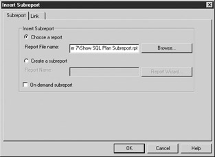
Figure 7-2: Link tab

Next, select the Link tab. Move %AUDSID from the Available Fields list into the Field(s) To Link To list. Set the Subreport Parameter Field To Use box to ?AUDSID (note that this should be ?AUDSID, not ?PM-%AUDSID). Clear the Select Data In Subreport Based On Field checkbox. The dialog box should look like Figure 7-3. Click OK and place the subreport in the report footer section.

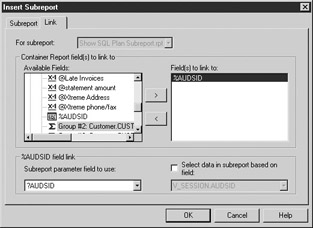
Figure 7-3: Insert Subreport dialog

Run the report. Log in to ORA2 if necessary. Because ORA2 is exactly the same database as ORA, the XTREME user can log on to both connections. Scroll to the last page of the report to view the plan subreport, as shown in Figure 7-4. This report is available as Chapter 7Account Statement with Plan Subreport.

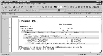
Figure 7-4: Statement of Account execution plan

The subreport uses Crystal’s hierarchical grouping, so the fields are indented a few characters to highlight children. The lightly shaded rows in the subreport show the actual filtering or joining conditions. The darker shaded rows show the SQL work area or PGA usage. Only some operations, such as sorting, require use of a work area. See the “PGA” section later in this chapter for more information about memory usage by work areas.

Note

When using this subreport with a report based on a stored procedure, modify the stored procedure to return the audit session ID in addition to the other required fields to use for linking, and modify the links in the subreport to use the SQL_ADDRESS and SQL_HASH_VALUE.

Note

This subreport works only for Oracle 9i. The V$SQL_PLAN and V$SQL_Workarea dynamic performance views do not exist in previous versions. The subreport works for all connection types, but be aware when changing the database location to an OLE DB type that the table aliases are slightly different for the dynamic performance views, so you must do a table-by-table change.

Optimizing the Environment

This chapter is concerned primarily with optimizing a single particular query. Optimizing the overall system is generally beyond the intended scope. However, it must be recognized that instance level parameters and resource consumption by other processes affect the performance of an individual query. Ideally, before attempting to optimize individual statements, the Oracle environment will be evaluated, decisions will be made about setting initialization parameters that influence query performance and memory usage, unnecessary anonymous PL/SQL blocks will be eliminated, and frequently used objects will be identified and pinned in memory.

Optimizer Initialization Parameters

The values of several initialization parameters affect the cost that the cost-based optimizer computes. Modifying these parameters can change the execution plan by causing some access methods to be more expensive than others. These parameters will affect all database queries, so care must be taken to ensure that improving reporting performance does not result in unacceptably degrading other areas.

CURSOR_SHARING

The CURSOR_SHARING parameter affects how statements are parsed. See Chapter 8 for a full description of this parameter.

DB_FILE_MULTIBLOCK_READ_COUNT

This parameter determines the number of blocks read in any multiblock read operation. Full table scans and index fast full scans use multiblock IO. The higher the value of DB_FILE_MULTIBLOCK_READ_COUNT, the more likely it will be that the optimizer will choose to do full table scans or index fast full scans instead of using other access methods.

HASH_AREA_SIZE

The size of this parameter affects the cost of a hash join operation. The larger the HASH_AREA_SIZE, the less costly a hash join will be. See the “PGA” section for details on setting this parameter.

HASH_JOIN_ENABLED

If this parameter is TRUE, the cost-based optimizer will consider using hash join operations. If it is FALSE, no hash joins will be done. The default value for this parameter for Oracle 8i and 9i is TRUE.

OPTIMIZER_INDEX_CACHING

This parameter influences the cost of index probing in nested loop operations and tells the optimizer to assume a particular percentage of index blocks are cached. A value of 100 indicates that the entire index is in the buffer cache. The default value for this parameter in Oracle 8i and 9i is 0.

OPTIMIZER_INDEX_COST_ADJ

This parameter reduces the estimated cost of index probing. A value of 100 means to use the normal cost. A value of 50 means to treat an index probe as if it costs 50 percent of the normal cost.

OPTIMIZER_MAX_PERMUTATIONS

This parameter controls the maximum number of join permutations that the cost-based optimizer will consider. Reducing it may reduce the parse time for queries containing many tables, but it may also cause the true optimal plan to never be considered.

OPTIMIZER_MODE

The OPTIMIZER_MODE parameter was covered in the “Oracle Optimizers” section. Oracle recommends using the cost-based optimizer.

PARTITION_VIEW_ENABLED

This parameter is useful when your environment contains partitioned tables. If it is TRUE, the optimizer will scan only the needed partitions based on join conditions or WHERE clauses.

QUERY_REWRITE_ENABLED

If TRUE, the optimizer will consider transparently rewriting queries to take advantage of existing materialized views. See Chapter 9 for an in-depth description. This parameter also determines whether function-based indexes are used; see the “Function-Based Index” section for more information.

SORT_AREA_SIZE

The larger the value of SORT_AREA_SIZE, the less the optimizer will estimate the cost of sort operations to be. See the “PGA” section for information about setting this parameter.

STAR_TRANSFORMATION_ENABLED

Setting the STAR_TRANSFORMATION_ENABLED optimizer parameter to TRUE enables the optimizer to cost star transformations using combinations of bitmap indexes. Star queries are used in a data warehouse environment where dimension and fact tables exist with bitmap indexes on those tables.

Memory Allocation

Memory use by an Oracle instance is divided among several caches or pools. Optimizing memory usage depends on allocating available memory to the pools in a manner that will produce the best overall performance. In-depth coverage of memory optimization is outside the scope of this book, but an overview is given to help the report writer understand how queries use server resources.

Buffer Cache

The buffer cache is where blocks of data are stored once they have been read from disk. All source data for a query is returned from the buffer cache. If a query requires data that is not already in the buffer cache, it is read from disk into the buffer cache for use. Queries should be optimized to require as few blocks as possible from the buffer cache, and the environment should be configured so that frequently used data can be found in the buffer cache, to avoid disk reads. The Crystal side optimization goal of returning as few records as possible will help optimize buffer cache use. The DBA will tune the buffer cache using tools such as the V$DB_CACHE_ADVICE and V$SYSSTAT dynamic performance views and monitor it over time.

Data in the buffer cache is aged out using a least recently used algorithm. As new data is placed at the most recently used end of the list, blocks at the least recently used end are dropped. Blocks read for full table scans and fast full index scans are an exception: they are placed at the least recently used end of the list with the rationale that the data will probably not be needed by other queries, should be aged out quickly, and should not force other blocks to be aged out.

The buffer cache can be segmented by using a KEEP or RECYCLE pool along with the DEFAULT pool. The KEEP and RECYCLE pools behave in exactly the same way as the DEFAULT pool because they all use a least recently used algorithm for aging blocks. However, the intention should be to store frequently accessed small segments in the KEEP pool and size the KEEP pool so that it is large enough to hold those items without aging them out. Large segments that are used infrequently should be stored in the RECYCLE pool where they will not cause undesired aging out in the DEFAULT or KEEP pools. The desired pool is set using the BUFFER_POOL keyword of the STORAGE clause for tables, indexes, and clusters. In a reporting environment, you might want to set the BUFFER_POOL to KEEP for small, frequently used lookup tables or frequently used indexes. You might also want to set the BUFFER_POOL to RECYCLE for large tables that are commonly accessed via full table scans.

Shared Pool and Large Pool

The shared pool contains the library cache, the dictionary cache, and other data. The dictionary cache stores data dictionary information, such as the column names that belong to a table, and is used heavily as almost every operation must verify catalog information. The library cache stores SQL statements, PL/SQL code, and their executable forms. Crystal Reports reads from the dictionary cache to create the table and field lists shown in the Database Expert. When Crystal Reports executes a query, that query is parsed using the dictionary cache, and the executable form is stored in the library cache. The dictionary and library caches, like other Oracle memory structures, use a least recently used algorithm to age items out of the cache. Oracle will dynamically resize the dictionary cache and library cache within the limits set for the shared pool.

The large pool can be created for use by the shared server, parallel query, or Recovery Manager to segregate those processes from other shared pool processes.

Reduce Parsing

The DBA will tune and monitor the shared pool. However, there are several things that report writers can do to help optimize use of the library cache. See Chapter 8 for more information.

Pin Frequently Used Cursors or PL/SQL Packages

Objects may be pinned in the shared pool so that they are never aged out. This can be useful if large objects are causing many other objects to be aged out due to lack of contiguous space. Pinning should be done immediately after instance startup both so that the pinned objects do not contribute to memory fragmentation and to guarantee their place in memory before any user might call them; this will eliminate any extra wait time on first execution.

Pinning is done using the DBMS_SHARED_POOL.KEEP procedure. Several object types may be pinned, including sequences and triggers, but report writers will be primarily concerned with SQL cursors and PL/SQL packages or procedures. If your most frequently used reports are based on stored procedures, and those stored procedures are in a package, pinning that package may be advantageous.

A procedure or package is pinned by executing a statement like the following:

DBMS_SHARED_POOL.KEEP(<>);

Pinning SQL cursors is more complex. The SQL cursor must exist in the shared pool, so it must have been previously parsed. You must determine the address and hash value of the cursor. Then you can pin the cursor using the following format:

DBMS_SHARED_POOL.KEEP(<>);

If you need to pin a cursor that is backing a report, it would be simpler to put that query in a stored procedure and pin the procedure or the package that contains it.

Eliminate Large Anonymous PL/SQL Blocks

Avoid an environment where large anonymous PL/SQL blocks are regularly executed. Large anonymous blocks are not likely to be sharable; hence, they will consume more space in the shared pool. If many similar blocks are being executed ad hoc or from scripts, consider creating PL/SQL parameterized procedures to reduce parsing and memory consumption. An anonymous block will be executed when a Crystal SQL Command is used that has multiple statements in it.

Qualify Object Names with the Schema Owner

When using SQL Commands, qualify the table or view name with the owner name whenever possible. Use XTREME.EMPLOYEE rather than EMPLOYEE. This will reduce the space used in the dictionary cache and speed the parsing process because the parser will not have to determine the proper schema.

PGA

Oracle 9i introduced automated management of several parameters that affect SQL execution for dedicated sessions, including HASH_AREA_SIZE, CREATE_BITMAP_AREA_SIZE and SORT_AREA_SIZE. Setting the PGA_AGGREGATE_TARGET to a value other than zero will cause the *_AREA_SIZE parameter values to be ignored for dedicated sessions in favor of dynamic manipulation by Oracle.

With the PGA_AGGREGATE_TARGET set, Oracle 9i will dynamically adjust the amount of memory allocated to the various work areas to optimize performance. The goal is to have as many executions as possible using an optimal work area size. One pass executions are usually acceptable but not as fast as optimal executions. Multipass executions should be avoided. The DBA should use the V$PGA_TARGET_ADVICE and the V$PGA_TARGET_ADVICE_HISTOGRAM to tune the PGA_AGGREGATE_TARGET parameter. The report writer can view work area usage in the execution plan subreport developed in the “Execution Plan Subreport” section. If you see reports running with multipass executions, consult your DBA.

Parallel Execution

Explaining the full details of parallel execution is beyond the scope of this book, but report writers should be aware of the possibility of parallel execution, especially when querying large tables. Parallel execution can improve the performance of large queries by distributing the work across multiple server processes. However, parallel execution requires more memory and CPU resources.

Certain initialization parameters must be set to enable a parallel execution environment, and there are two possible methods of implementing parallel query execution. The DBA can set the PARALLEL option on tables and indexes to cause parallel execution for all operations against those objects. Alternatively, a SELECT statement can be written with the PARALLEL hint, which will force parallel execution for that particular query.

Table Partitioning

Table partitioning breaks the physical storage of tables into chunks or partitions that are transparent to any user querying the database. Users do not need to know anything about the partition status of any tables. However, if a table is partitioned and a query requires data only from some partitions, the query performance may be improved. The report writer has no direct method of creating partitioned tables because that is a function of the DBA and must be done at table creation. However, the report writer should be aware that tables can be partitioned and that partitioning may improve query performance on large tables or indexes.

There are several types of partitioning; a common type is partitioning by date. Suppose that in the sample data, the Orders table was very large. If you partitioned it by Order_Date or a range of Order_Dates, then reports that were always run for today or this month would probably see a performance gain.

Dynamic Sampling

Dynamic sampling is a new feature of Oracle 9i release 2. Dynamic sampling allows the optimizer to sample data from tables to make estimates about cardinality and selectivity. This can be helpful in situations where there are no statistics gathered, the statistics are old, or the statistics are not desirable for some other reason. The optimizer determines whether dynamic sampling would be useful for each query, and the level of sampling is controlled by the initialization parameter OPTIMIZER_DYNAMIC_SAMPLING. The optimizer hint DYNAMIC_SAMPLING customizes the sampling for a particular query.

Optimizing the Execution Plan

Optimizing an execution plan can involve several methods. This section covers various general tips to improve query performance, as well as optimizer hints that can be set for an individual query, indexing to improve performance, and using stored outlines.

Tips

Some general tips for optimization of execution plans are to make sure that statistics have been gathered appropriately so that the cost-based optimizer has up-to-date information and to use the execution plan subreport or Explain Plan to view the execution plan for a report query, then check the plan for any of the following conditions.

Eliminate Cartesian Products

If the execution plan shows a Cartesian product, there is probably a missing table linking condition. On rare occasions, a Cartesian product can be intentional and necessary.

Avoid Full Table Scans

Full table scans should be avoided unless the tables are small, the query returns more than 5 percent to 10 percent of the rows, you are using parallel execution, or in some cases where a hash join is used. For some reports, a large portion of rows will be returned, so full table scans may be appropriate.

Join Order

An important tuning goal is to filter out as many records as you can as soon as possible in the execution plan. Review the execution plan from the leaf operations to the final operations. Verify that the data source with the most selective filter is used first, followed by the source with the next most selective filter, and so on.

Optimal Join Method

The optimal join method, when a small number of rows will be returned, is usually nested loops. Other methods might be more appropriate when larger numbers of rows are returned.

Appropriate Table Access Methods

For tables that have filtering conditions in the WHERE clause, if that filtering will return a small number of rows from the table, you should expect to see the use of an index. If an index is not being used in this circumstance, then you should investigate why. If there is no filtering or the filtering is not very selective, you might expect to see a full table scan.

Use Equijoins

Equijoins, joins based on equality conditions, are more efficient than nonequijoins, which are fairly uncommon but necessary for some queries. If you see a join condition containing anything other than an equal sign, verify that it is appropriate.

Avoid Expressions in Join Conditions and WHERE Clauses

If the join condition or filter condition contains an expression instead of a simple column name, indexes cannot be used unless the expression has an equivalent function-based index. Be aware of implicit type conversions where Oracle will rewrite the query to contain the appropriate conversion function. For instance, if you have a filtering condition such as the following where ColA is VARCHAR2:

WHERE ColA=100

Oracle will convert it as shown and no index can be used:

WHERE TO_NUMBER(ColA)=100

To avoid this, rewrite the condition as shown next, assuming the format string is appropriate and any index on ColA can be used:

WHERE ColA=TO_CHAR(100,'L99G999D99MI')

When functions such as NVL are used in filtering conditions, they can sometimes be rewritten to avoid the use of the function. For example, the following condition:

WHERE NVL(Col1,100)=100

can be rewritten as shown to preserve the use of indexes:

WHERE (Col1=100 OR Col1 IS NULL)

Use Views Appropriately

When a view is used in a query, verify that it is necessary. For instance, if a view containing joins is used but all fields in the SELECT clause are from one table only, it would be more efficient to use the underlying table. There are some organizations in which views are used to insulate the reports from changes in the underlying database. In this case, views should be available that are based on single tables, in addition to any special purpose views containing joins. The single table views should then be used for reports on individual tables, and the optimizer will rewrite the query to use the table.

Avoid Joining Views

The optimizer will attempt to rewrite views to use underlying tables when possible, but using a query that joins views may make this rewrite impossible. In this case, a view may have to be instantiated to complete the query, which will cause heavy resource usage. If you have a report that contains a view joined to another view, it’s better to create a new view containing the data you need and eliminate the view joins.

Use CASE Statements

This tip is not strictly about optimizing an execution plan. Sometimes multiple queries are used to return different aggregations of the same data. For instance, say that you need the count of employees whose salary is less than $30,000, and you also need the count of employees whose salary is between $30,000 and $60,000. Instead of creating two queries, one query with a CASE statement could be used, reducing the number of times that the same data needs to be read.

Optimizer Hints

Optimizer hints are keywords embedded in the SELECT statement that direct the optimizer to use a particular join order, join method, access path, or parallelization. The hint follows the SELECT statement. If a query is compound, with multiple SELECT statements, each can have its own hint. Optimizer hints can be used in SQL Commands, stored procedures, and view definitions.

Only commonly used hints for SELECT statements are covered.

The syntax for specifying hints is shown next:

SELECT /*+ hint [text] [hint[text]]... */

Optimizer Mode Hints

Optimizer mode hints are those hints that influence how the cost-based optimizer will cost the statement. Note that if the FIRST_ROWS, FIRST_ROWS(n), or ALL_ROWS optimizer hints are used, the cost-based optimizer will be used even if statistics do not exist.

FIRST_ROWS(n)

SELECT /*+ FIRST_ROWS(n) */ …

The FIRST_ROWS(n) hint tells the optimizer to pick the execution plan that returns the first n rows the fastest. N can be any positive integer. This differs from the corresponding First Rows optimizer mode that allows a limited set of values for n. The FIRST_ROWS(n) hint will be ignored if the statement contains any operation that requires returning all rows before selecting the first n. Such operations include GROUP BY, ORDER BY, aggregation, UNION, and DISTINCT. FIRST_ROWS(n) has limited usage for Crystal Reports queries because few report queries lack at least an ORDER BY clause.

Note

The FIRST_ROWS(n) optimizer hint is new in Oracle 9i.

FIRST_ROWS

FIRST_ROWS is equivalent to FIRST_ROWS(1).

ALL_ROWS

SELECT /*+ ALL_ROWS */ …

The ALL_ROWS hint causes the optimizer to optimize for maximum throughput, to return all rows as fast as possible.

CHOOSE

SELECT /*+ CHOOSE */ …

The CHOOSE hint tells Oracle to use the cost-based optimizer if any table in the query has statistics and to use the rule-based optimizer if no statistics exist.

RULE

SELECT /*+ RULE */ …

The RULE hint instructs Oracle to use the rule-based optimizer even if statistics exist.

Access Path Hints

Access path hints tell the optimizer which access path it should use. If the hinted access path is unavailable, the hint is ignored. For these hints, the table name must be given. If an alias for the table name exists, the alias should be used in the hint.

FULL

SELECT /*+ FULL (table_name or alias) */ …

The FULL hint forces a full table scan. A full table scan can be more efficient than an index scan if a large portion of the table rows need to be returned because of the way data is read for a full table scan versus an index scan. In a full table scan, multiple blocks are read simultaneously. In an index scan, one block is read at a time. Whether using a full scan is better than an index scan depends on many things, including the speed of the hardware, the DB_FILE_MULTIBLOCK_READ_COUNT, the DB_BLOCK_SIZE, and the way the index values are distributed. If your query returns more than 5 to 10 percent of the rows and the optimizer chooses to use an index, you may want to investigate the results of forcing a full table scan.

ROWID

SELECT /*+ ROWID (table_name or alias) */ …

A ROWID hint forces the table to be scanned by ROWID.

INDEX

SELECT /*+ INDEX (table_name or alias [index_name1
 [index_name2…]]) */ …

The INDEX hint forces an index scan on the table listed. If no index names are given, the optimizer will use the index with the least cost. If one index name is given, the optimizer will use that index. If multiple index names are given, the optimizer will use the index from the list that has the least cost.

INDEX_ASC

SELECT /*+ INDEX_ASC (table_name or alias [index_name1
 [index_name2…]]) */ …

The INDEX_ASC hint is currently identical to the INDEX hint. It forces an index scan in ascending order.

INDEX_COMBINE

SELECT /*+ INDEX_COMBINE (table_name or alias
 [bitmap_index_name1
 [bitmap_index_name2…]]) */ …

INDEX_COMBINE is similar to INDEX but forces a bitmap index to be used.

INDEX_JOIN

SELECT /*+ INDEX_JOIN (table_name or alias
 [join_index_name1
 [join_index_name2…]]) */ …

INDEX_JOIN forces the optimizer to use an index join on the listed tables.

INDEX_DESC

SELECT /*+ INDEX_DESC (table_name or alias [index_name1
 [index_name2…]]) */ …

INDEX_DESC is similar to INDEX, but if the statement requires a range scan, the INDEX_DESC hint will force the range to be scanned in reverse order.

INDEX_FFS

SELECT /*+ INDEX_FFS (table_name or alias [index_name1
 [index_name2…]]) */ …

INDEX_FFS forces a fast full index scan instead of a full table scan.

NO_INDEX

SELECT /*+ NO_INDEX (table_name or alias [index_name1
 [index_name2…]]) */ …

NO_INDEX removes the listed indexes from the compiler’s consideration. If no index names are given, none of the available indexes will be used. If one or more index names are given, only those indexes will not be considered and any other existing indexes can be used.

CLUSTER

SELECT /*+ CLUSTER(table_name or alias) */ …

The CLUSTER hint forces a cluster scan of the specified table. This hint can only be used with tables that are part of a cluster.

HASH

SELECT /*+ HASH(table_name or alias) */ …

The HASH hint forces a hash scan of the specified table. This hint can only be used with tables that are part of a cluster.

AND_EQUAL

SELECT /*+ AND_EQUAL(table_name or alias index_name1 index_name2 
[[index_name3 [index_name4]] [index_name5]]) */ …

The AND_EQUAL hint forces the optimizer to combine index scans for the listed table using from two to five of its single column indexes.

Join Order Hints

Join order hints let you tell the optimizer in what order the tables should be joined.

ORDERED

SELECT /*+ ORDERED */ …

ORDERED forces the optimizer to join the tables in the order they are listed in the FROM clause. Using the new Oracle 9i join syntax, the same result can be obtained without using hints.

STAR

SELECT /*+ STAR */ …

The STAR hint forces a star query plan to be used, if possible. This hint is used in data warehouse environments.

Join Operation Hints

The join operation hints suggest join methods for tables in the query.

Several special purpose join operation hints are not covered here, including DRIVING_SITE, HASH_AJ, MERGE_AJ, NL_AJ, HASH_SJ, MERGE_SJ, and NL_SJ. For information about these hints, refer to Oracle documentation.

USE_NL

SELECT /*+ ORDERED USE_NL (table_name or alias) */ …

The USE_NL hint forces a nested loop join and may cause the first rows of a query to be returned faster than they would be if a merge join was used. The ORDERED hint should always be used with this hint, and the table listed in the hint must be the inner table of a nested loop join.

USE_MERGE

SELECT /*+ USE_MERGE (table_name or alias) */ …

The USE_MERGE hint forces a merge join of the given table and may cause the entire query result to be returned faster than if a nested table join was used. The ORDERED hint should always be used with this hint, and the table listed in the hint will be merged to the result set of any joins preceding it in the order.

USE_HASH

SELECT /*+ USE_HASH (table_name or alias) */ …

The USE_HASH hint will force the listed table to be joined using a hash join.

LEADING

SELECT /*+ LEADING (table_name or alias) */ …

The LEADING hint forces the table listed to be first in the join order. LEADING is overridden by an ORDERED hint.

Parallel Hints

The work involved in processing a query can be broken into pieces, and the pieces can be executed simultaneously. This is called parallel execution. Parallel query execution is used if the tables involved in the query have their parallel option set or if a parallel hint is in the query, assuming that other initialization parameters that govern parallel execution are set.

Note that parallel execution is not the same thing as partitioning. Partitioned tables are broken into pieces for storage and can influence query execution because only required partitions may need to be read. Parallel execution, however, refers to the number of server processes that are working on the query.

PARALLEL

SELECT /*+ PARALLEL(table_name or alias[,degree_of_parallelism]) */ …

If no degree of parallelism is given, the system default based on initialization parameters will be used.

NOPARALLEL

SELECT /*+ NOPARALLEL(table_name or alias) */ …

If a table is used that has its parallel option set, this hint will override that and cause the query to execute without parallelism.

Three other parallel hints exist: PQ_DISTRIBUTE allows you to fine-tune the distribution of parallel join operations among query servers; PARALLEL_INDEX can be used with partitioned indexes to set the number of Oracle Real Application Cluster instances and the number of query servers working on those instances; and NO_PARALLEL_INDEX instructs the optimizer to not use a parallel index scan on the listed table and/or index.

Other Hints

There are several other hints that do not fit into the preceding categories. A few of them are covered here. See Oracle documentation for any that you do not find here.

CACHE

SELECT /*+ CACHE (table_name or alias) */ …

As discussed previously, when a full table scan is performed, the blocks read are placed at the least recently used end of the buffer so that they will age out quickly. The CACHE hint, however, causes the blocks to be placed at the most recently used end so that they will not age out quickly. This might be useful for small lookup tables that are read frequently with full table scans, but small tables are automatically cached in Oracle 9i release 2.

CURSOR_SHARING_EXACT

SELECT /*+ CURSOR_SHARING_EXACT */ …

If the CURSOR_SHARING initialization parameter is set to FORCE or SIMILAR, using the CURSOR_SHARING_EXACT hint will override that behavior for the query containing the hint.

Note

CURSOR_SHARING_EXACT is new in Oracle 9i.

DYNAMIC_SAMPLING

SELECT /*+ DYNAMIC_SAMPLING ([table_name or alias] sampling_level) */ …

The DYNAMIC_SAMPLING hint allows the optimizer to gather sample statistics for the query to help in determining cardinality and selectivity. If a table name is supplied, the sampling will be done only for that table. If no table name is supplied, sampling is done for the whole query, as indicated by the sampling level. The sampling level is a number from 0 to 10: 0 turns off sampling; 1 is the default value and indicates that sampling will be done on unanalyzed, nonindexed tables that are joined to other tables or used in subqueries and that have more than 32 blocks of data. Thirty-two blocks will be sampled. Setting the sampling level higher makes the sampling more aggressive and more likely. See Oracle documentation for a full description of the levels.

Note

The DYNAMIC_SAMPLING hint is new in Oracle 9i.

Indexing

Proper database indexing is a complex topic and has widespread effects. The DBA, application developers, and report writers must coordinate indexing decisions so that end users get the best overall performance. A report writer might commonly notice that the query execution plan does not use an index where expected. The report writer would then discuss the matter with the DBA and/or the application developers, so that an optimal indexing decision could be made.

There are several key places where indexing will speed query execution. Indexing the columns used in WHERE clauses will speed query execution. Indexing the columns used to join tables will also speed query execution. Reordering columns in concatenated indexes so that the most selective fields are first may speed query execution. If an index is not selective, adding a column to it may increase its selectivity (the selectivity of an index refers to the number of rows with the same value). The fewer the number of rows with the same value, the higher the selectivity of the index.

Nonselective indexes probably will not affect SELECT performance because the optimizer will probably not use them, but they will be detrimental to data manipulation statements. The DBA should monitor index usage and drop any unnecessary unused indexes. Be aware that indexing will have a negative impact on DML operations, so avoid indexing columns that are frequently updated.

B-tree Index

The default Oracle index is a B-tree index. B-tree indexes should be used in most cases where indexing is required and cardinality is high.

Function-Based Index

Function-based indexes allow you to create indexes on expressions. This speeds query execution when an expression is used often in the WHERE clause or ORDER BY clause. For example, consider the Last_Name column in the Employee table. A regular index created on Last_Name would be useful when a SELECT statement with the following WHERE clause was issued:

SELECT
…
WHERE Last_Name='King';

That index would be useless if the query was as follows:

SELECT
…
WHERE UPPER(Last_Name)='KING';

However, if a function-based index was created on the expression UPPER(Last_Name), it could be used in the previous query.

The database initialization parameter, QUERY_REWRITE_ENABLED must be true, or the equivalent session parameter must be true for function-based index use. By default, function-based indexes can only be created for built-in functions. To enable the use of user-defined functions, you must set the QUERY_REWRITE_INTEGRITY parameter to something other than its default value of ENFORCED.

Function-based indexes precompute expressions that are commonly used in WHERE clauses. Suppose that the month of order is used in many reports, so that many reports have clauses like the following two:

WHERE Extract(Month from Order_Date) = :Order_Month


ORDER BY Extract(Month from Order_Date)

A function-based index on the expression Extract(Month from Order_Date) would improve query performance.

Index Organized Tables

Index organized tables are Oracle tables where the entire row data is stored in the index. Hence, the entire table, not just the index, is always in physical order by the primary key. This structure is similar to some desktop databases such as Access or Paradox, where the rows are maintained in primary key order when inserts, deletes, or updates are made. Index organized tables can speed query execution if many queries use exact match or range searches of the primary key.

Bitmap Index

A bitmap index is appropriate for table columns with few distinct values and a large number of rows, but it can be costly to keep updated if there is frequent, nonbulk updating. Bitmap indexes are frequently used in data warehousing environments, where they help speed the processing of queries with complex WHERE clauses. In the XTREME sample data, a column such as Customer.Country is a candidate for a bitmap index because it has few distinct values.

Bitmap indexes require less storage than B-tree indexes. Bitmap indexes on single columns can be combined for use in WHERE clauses that use more than one bitmap indexed column. Bitmap indexes cannot be used to enforce referential integrity constraints.

Bitmap Join Index

Bitmap join indexes are used in data warehousing environments to effectively prejoin tables. The bitmap join index contains entries for the join columns and the ROWIDs of the corresponding rows.

Note

Bitmap join indexes are new in Oracle 9i.

Other Index Types

Other indexing methods are available. Domain indexes are indexes built using a user-defined index type. Domain indexes are usually supplied as part of an Oracle cartridge and enable indexing of complex user-defined data types. Clusters and hash clusters speed access to tables that are frequently queried together via joins.

Stored Outlines

An execution plan can be stored so that the SQL statement will always use that plan. If a stored outline exists, the cost-based optimizer will use it even if current conditions dictate a different plan. Stored outlines should be used with care, however, because they can result in performance degradation over time. See Oracle documentation for more detail on creating and using stored outlines.

This chapter described the Oracle optimizers and execution plans. A subreport for displaying report query execution plans was created, and tips were given for optimizing the execution plan. The next chapter will explain SQL statement parsing and the impact of parsing on a reporting environment and give suggestions for parse reduction.