Spatial Image Filtering

As the word filtering suggests, most of the methods described in this section are used to improve the quality of the image. In general, these methods calculate new pixel values by using the original pixel value and those of its neighbors. For example, we can use the equation

Equation 4.12

which looks very complicated. Let's start from the left: Eq. (4.12) calculates new pixel values s out by using an m x m array. Usually, m is 3, 5, or 7; in most of our exercises we use m = 3, which means that the original pixel value s in and the values of the eight surrounding pixels are used to calculate the new value. k is defined as k = ( m “ 1)/2.

The values of these nine pixels are modified with a filter kernel

Equation 4.13

As you can see in Eq. (4.12), the indices u and v depend upon x and y with k = ( m “ 1)/2. Using indices x and y , we can write

Equation 4.14

which specifies the pixel itself and its eight surrounding neighbors.

The filter kernel moves from the top-left to the bottom-right corner of the image, as shown in Figure 4.19. To visualize what happens during the process, do Exercise 4.6:

Figure 4.19. Moving the Filter Kernel

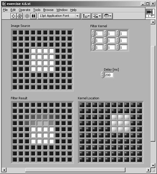
Exercise 4.6: Filter Kernel Movement.

Visualize the movement of a 3 x 3 filter kernel over a simulated image and display the results of Eq. (4.12). Figures 4.19 and 4.20 show a possible solution.

In this exercise I simulated the image with a 10 x 10 array of color boxes. Their values have to be divided by 64 k to get values of the 8-bit gray-scale set. The pixel and its eight neighbors are extracted and multiplied by the filter kernel, and the resulting values are added to the new pixel value.

 

Figure 4.20. Diagram of Exercise 4.6

The process described by Eq. (4.12) is also called convolution ; that is why the filter kernel may be called convolution kernel .

You may have noticed that I did not calculate the border of the new image in Exercise 4.6; the resulting image is only an 8 x 8 array. In fact, there are some possibilities for handling the border of an image during spatial filtering:

• The first possibility is exactly what we did in Exercise 4.6: The resulting image is smaller by the border of 1 pixel.
• Next possibility: The gray-level values of the original image remain unchanged and are transferred in the resulting image.
• You can also use special values for the new border pixels; for example, 0, 127, or 255.
• Finally, you can use pixels from the opposite border for the calculation of the new values.

Kernel Families

LabVIEW provides a number of predefined filter kernels; it makes no sense to list all of them in this book. You can find them in IMAQ Vision Help: In a LabVIEW VI window, select Help / IMAQ Vision... and type " kernels " in the Index tab.

Nevertheless, we discuss a number of important kernels using the predefined IMAQ groups. To do this, we have to build a LabVIEW VI that makes it possible to test the predefined IMAQ Vision kernels as well as the manually defined kernels.

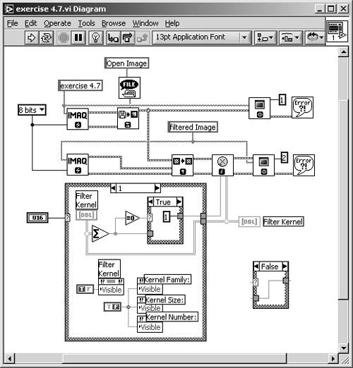
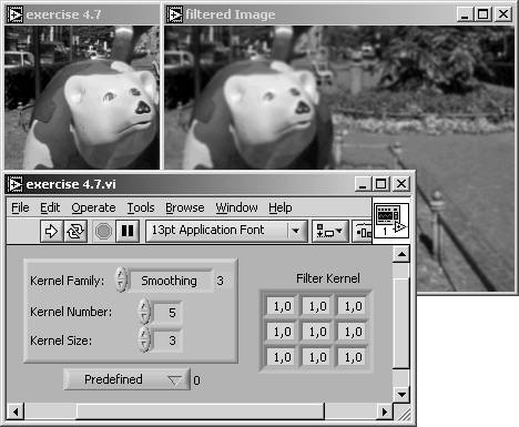
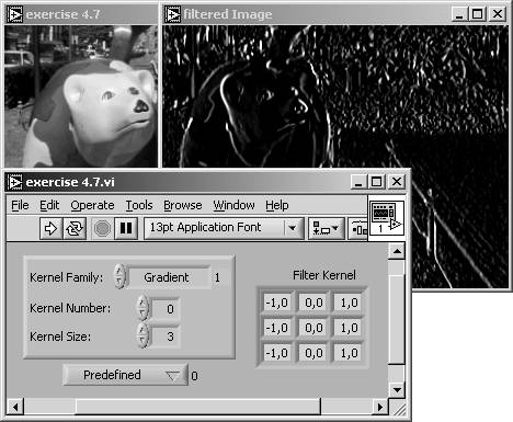
Exercise 4.7: IMAQ Vision Filter Kernels.

In this exercise VI, you will be able to visualize the built-in IMAQ Vision filters, and this allows you to define your own 3 x 3 kernels. Figure 4.21 shows the front panel: The Menu Ring Control (bottom-left corner) makes it possible to switch between Predefined and Manual Kernel. I used Property Nodes here to make the unused controls disappear.

Next, let's look at the diagram (Figure 4.22). The processing function we use here is IMAQ Convolute ; the predefined kernels are generated with IMAQ GetKernel . So far, so good; but if we use manual kernels, we have to calculate a value called Divider, which is nothing more than 1/ m 2 in Eq. (4.12).

Obviously, 1/ m 2 is not the correct expression for the divider if we want to keep the overall pixel brightness of the image. Therefore, we must calculate the sum of all kernel elements for the divider value; with one exception [2] of course, 0. In this case we set the divider to 1. [3]

[2] This happens quite often, for example consider a kernel .

[3] Note that if you wire a value through a case structure in LabVIEW, you have to click once within the frame.

 

Figure 4.21. Visualizing Effects of Various Filter Kernels

Figure 4.22. Diagram of Exercise 4.7

The four filter families which you can specify in Exercise 4.7 (as well as in the Vision Builder) are:

• Smoothing
• Gaussian
• Gradient
• Laplacian

Image Smoothing

All smoothing filters build a weighted average of the surrounding pixels, and some of them also use the center pixel itself.

Filter Families: Smoothing

A typical smoothing kernel is shown in Figure 4.23. Here, the new value is calculated as the average of all nine pixels using the same weight:

Equation 4.15

 

Figure 4.23. Filter Example: Smoothing (#5)

Other typical smoothing kernels are or Note that the coefficient for the center pixel is either 0 or 1; all other coefficients are positive.

Filter Families: Gaussian

The center pixel coefficient of a Gaussian kernel is always greater than 1, and thus greater than the other coefficients because it simulates the shape of a Gaussian curve. Figure 4.24 shows an example.

Figure 4.24. Filter Example: Gaussian (#4)

More examples for Gaussian kernels are or

Both smoothing and Gaussian kernels correspond to the electrical synonym " low-pass filter" because sharp edges, which are removed by these filters, can be described by high frequencies.

Edge Detection and Enhancement

An important area of study is the detection of edges in an image. An edge is an area of an image in which a significant change of pixel brightness occurs.

Filter Families: Gradient

A gradient filter extracts a significant brightness change in a specific direction and is thus able to extract edges rectangular to this direction. Figure 4.25 shows the effect of a vertical gradient filter, which extracts dark-bright changes from left to right.

Figure 4.25. Filter Example: Gradient (#0)

Note that the center coefficient of this kernel is 0; if we make it equal to 1 (as in Figure 4.26), the edge information is added to the original value. The original image remains and the edges in the specified direction are highlighted.

Figure 4.26. Filter Example: Gradient (#1)

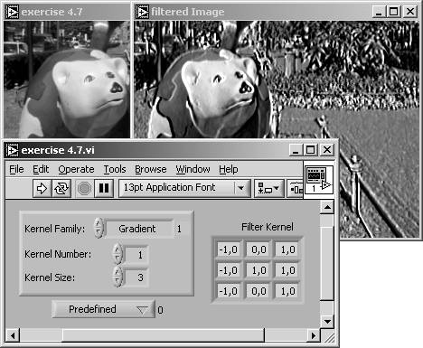
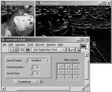
Figure 4.27 shows the similar effect in a horizontal direction (dark-bright changes from bottom to top).

Figure 4.27. Filter Example: Gradient (#4)

Gradient kernels like those in Figure 4.25 and Figure 4.27 are also known as Prewitt filters or Prewitt kernels . Another group of gradient kernels, for example, are called Sobel filters or Sobel kernels . A Sobel kernel gives the specified filter direction a stronger weight.

In general, the mathematic value gradient specifies the amount of change of a value in a certain direction. The simplest filter kernels, used in two orthogonal directions, are

Equation 4.16

 

resulting in two images, I x = ( s x ( x,y )) and I y = ( s y ( x,y )). Value and direction of the gradient are therefore

Equation 4.17

 

Filter Families: Laplacian

All kernels of the Laplacian filter group are omnidirectional; that means they provide edge information in each direction. Like the Laplacian operator in mathematics, the Laplacian kernels are of a second-order derivative type and show two interesting effects:

• If the sum of all coefficients is equal to 0, the filter kernel shows all image areas with a significant brightness change; that means it works as an omnidirectional edge detector (see Figures 4.28 and 4.30).
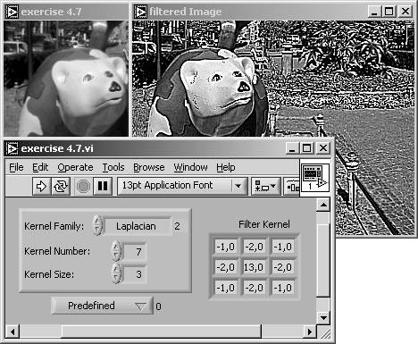
• If the center coefficient is greater than the sum of the absolute values of all other coefficients, the original image is superimposed over the edge information (see Figures 4.29 and 4.31).

Figure 4.28. Filter Example: Laplace (#0)

Figure 4.29. Filter Example: Laplace (#1)

Figure 4.30. Filter Example: Laplace (#6)

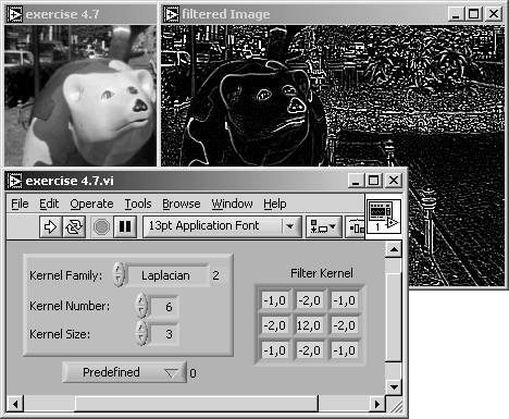
Figure 4.31. Filter Example: Laplace (#7)

Both gradient and Laplacian kernels correspond to the electrical synonym "high-pass filter." The reason is the same as before; sharp edges can be described by high frequencies.

Frequency Filtering