Compression Techniques

The following section discusses some techniques that make transport and storage of data, especially of image data, more effective. It distinguishes between lossless compression techniques, which enable the reconstruction of the image without any data loss and lossy compression techniques. Two good books for the details, from which most of the algorithm descriptions are taken, are [28] and [29].

Table 3.4. Comparison of Digital Camera Interfaces

	IEEE 1394	USB 2.0	Camera Link
Max. data rate:	800 Mbit/s	480 Mbit/s	~ 7.14 Gbit/s
Architecture:	Peer-to-peer	Host oriented	Peer-to-peer
Max. devices:	63	127 (incl. hubs)
Max. cable length:	4.50 m	5 m	~ 10 m
Total poss. distance:	72 m	30 m	~ 10 m
Wires for 8 bit/pixel:	4	2	10
Bidirectional comm.:	Yes (asynchronous)	Yes (asynchronous)	Additional channel
Power supply:	8-40 V, 1.5 A	5 V, 500 mA

Figure 3.30 illustrates the most common compression techniques and algorithms. According to [29], algorithms for compressing symbolic data such as text or computer files are called lossless compression techniques, whereas algorithms for compressing diffuse data like image and video content (when exact content is not important) are called lossy compression techniques.

Figure 3.30. Compression Techniques and Algorithms

Lossless Compression

This section deals with methods and standards by which uncompressed data can be exactly recovered from the original data. Medical applications especially need lossless compression techniques; for example, consider digital x-ray images, where information loss may cause diagnostic errors.

The following methods can also be used in combination with other techniques, sometimes even with lossy compression. Some of them we discuss in the section dealing with image and video formats.

Run Length Encoding (RLE)

Consider a data sequence containing many consecutive data elements, here named characters . A block of consecutive characters can be replaced by a combination of a byte count and the character itself. For example:

AAAAAAAAAAAA

(uncompressed)

is replaced with

12A

(compressed).

Of course, this is an example in which the data compression by the RLE algorithm is obvious. In the following example, the data compression is significantly lower:

AAAAABBBCCCCD

(uncompressed)

is replaced with

5A3B4C1D

(compressed).

The RLE algorithm is very effective in binary images containing large "black" and "white" areas, which have long sequences of consecutive 0s and 1s.

Huffman Coding

The Huffman coding technique [5] is based on the idea that different symbols of a data source s i occur with different probabilities p i , so the self-information of a symbol s i is defined as

[5] Developed by D. A. Huffman in 1952.

Equation 3.1

 

If we assign short codes to frequently occurring (more probable) symbols and longer codes to infrequently occurring (less probable) symbols, we obtain a certain degree of compression. Figure 3.31 shows an example.

Figure 3.31. Example of Huffman Coding

The Huffman code is generated in the following four steps:

1. Order the symbols s j according to their probabilities p j .
2. Replace the two symbols with the lowest probability p j by an intermediate node, whose probability is the sum of the probability of the two symbols.
3. Repeat step 2 until only one node with the probability 1 exists.
4. Assign codewords to the symbols according to Figure 3.31.

Obviously, the code can be easily decoded and no prefix for a new code word is needed. For example, we can decode the code sequence

10000001010001

(Huffman coded)

to

AECBD

(decoded)

by simply looking for the 1s and counting the heading 0s. If no 1 appears, then four 0s are grouped to E.

By the way, the principle of the Huffman coding is used in the Morse alphabet; the shortest symbols, the dot () and the dash (-) represent the most common letters (at least, the most common letters in Samuel Morse's newspaper) "e" and "t," respectively.

Lempel-Ziv Coding

This is another group of compression methods, invented by Abraham Lempel and Jacob Ziv in the late 1970s, consisting of algorithms called LZ77, LZ78, and some derivatives, for example, LZW (from Lempel-Ziv-Welch), and some adaptive and multidimensional versions. Some lossy versions also exist. Here, I describe the priniciple of LZ77, which is also used in some text-oriented compression programs such as zip or gzip .

Figure 3.32 shows the principle. The most important part of the algorithm is a sliding window, consisting of a history buffer and a lookahead buffer [6] that slide over the text characters. The history buffer contains a block of already decoded text, whereas the symbols in the lookahead buffer are encoded from information in the history buffer. [7]

[6] The sizes of the buffers in Figure 3.32 are not realistic. Typically, the history buffer contains some thousand symbols, the lookahead buffer 1020 symbols.

[7] Therefore, such methods sometimes are called dictionary compression .

Figure 3.32. Lempel-Ziv Coding Example (LZ77 Algorithm)

The text in the windows in Figure 3.32 is encoded as follows :

1. Each of the symbols in the history buffer is encoded with 0 , where 0 indicates that no compression takes place and is the ASCII character value.
2. If character strings that match elements of the history buffer are found in the lookahead buffer (here: PROCESS and IMAGE), they are encoded with a pointer of the format 1 . For PROCESS, this is 1 <11><7> (decimal).
3. E and S are encoded according to item 1.
4. The resulting pointer for IMAGE is 1 <27><5> (decimal).
5. Finally, S is encoded according to items 1 and 3.

The compression rate in this example is not very high; but if you consider that usually the history buffer is significantly larger than in our example, it is easy to imagine that compression can be much higher.

Arithmetic Coding

The codes generated in the previous sections may become ineffective if the data contains one or more frequently occuring symbols (that means, with a high probability p i ). For example, a symbol S occurs with the probability p S = 0.9. According to Eq. (3.1), the self-information of the symbol (in bits) is

Equation 3.2

 

which indicates that only 0.152 bits are needed to encode S . The lowest number of bits a Huffman coder [8] can assign to this symbol is, of course, 1. The idea behind arithmetic coding is that sequences of symbols are encoded with a single number. Figure 3.33 shows an example.

[8] This is why Huffman coding works optimally for probabilities that are negative powers of 2 (1/2, 1/4, ...).

Figure 3.33. Arithmetic Coding Example

The symbol sequence to be encoded in this example is VISIO. [9] In a first step, the symbols are ordered (here, alphabetically ) and their probability in the sequence is calculated. A symbol range of 0.01.0 is then assigned to the whole sequence and, according to their probabilities, to each symbol (top-right corner of Figure 3.33).

[9] I tried to use VISION, but as you will see, sequences with five symbols are easier to handle.

Then the entire coding process starts with the first symbol, V. The related symbol range is 0.81.0; multiplied by the starting interval width of 1.0 a new message interval is generated. The next symbol is I; it has a symbol range of 0.00.4. Multiplication by the previous message interval width 0.2 and addition to the previous message interval left border lead to the new message interval 0.800.88. This procedure is repeated until all of the symbols have been processed .

The coded result can be any number in the resulting message interval and represents the message exactly, as shown in the decoding example in Figure 3.34. (In this example, I chose 0.85100.)

Figure 3.34. Arithmetic Decoding Example

To get the first symbol, the entire code number is checked for the symbol range it is in. In this case, it is the range 0.81.0, which corresponds to V. Next, the left (lower) value from this range is subtracted from the codeword, and the result is divided by the symbol probability, leading to

 

the new codeword, which is in the range 0.00.4 corresponding to I, and so on.

Table 3.5 compares the lossless compression algorithms discussed above.

Table 3.5. Comparison of Lossless Compression Algorithms

Coding:	RLE	Huffman	LZ77	Arithmetic
Compression ratio:	very low	medium	high	very high
Encoding speed:	very high	low	high	very low
Decoding speed:	very high	medium	high	very low

MH, MR, and MMR Coding

These methods are especially used in images. They are closely related to the techniques already discussed, so we discuss them only briefly here. See [28] [29].

• Modified Huffman (MH) coding treats image lines separately and applies an RLE code to each line, which is afterwards processed by the Huffman algorithm. After each line an EOL (end of line) code is inserted for error detection purposes.
• Modified READ (MR; READ stands for relative element address designate ) coding uses pixel values in a previous line as predictors for the current line and then continues with MH coding.
• Modified modified READ (MMR) simply uses the MR coding algorithm without any error mechanism, again increasing the compression rate. MMR coding is especially suitable for noise-free environments.

Lossy Compression

The borders between lossy compression methods and image standards are not clear. Therefore, I focus on the relevant compression standard for still images, JPEG, together with a short description of its main method, discrete cosine transform, and on its successor, JPEG 2000, which uses wavelet transform.

Discrete Cosine Transform (DCT)

Most lossy image compression algorithms use the DCT. The idea is to transform the image into the frequency domain, in which coefficients describe the amount of presence of certain frequencies in horizontal or vertical direction, respectively.

The two-dimensional (2-D) DCT we use here is defined as

Equation 3.3

 

with k , l = 0, 1, ... , 7 for an 8 x 8 image area, x ij as the brightness values of this area, and

Equation 3.4

 

The resulting coefficients y kl give the corresponding weight for each discrete waveform of Eq. (3.3), so the sum of these results is again the (reconstructed) image area.

An important drawback of this calculation is that the effort rises with ( n log ( n )), therefore more than linear. This is why the original image is structured in 8 x 8 pixel areas, called input blocks . Figure 3.35 shows this procedure for an image from Chapter 1.

Figure 3.35. 8 x 8 DCT Coefficients

Figure 3.35 also shows the brightness information of the input block ( x ij ) and the result of the DCT coefficient calculation ( y kl ) according to Eq. (3.3). This calculation can be done by the VI created in Exercise 3.3.

Exercise 3.3: Calculating DCT Coefficients.

Create a LabVIEW VI that calculates the 8 x 8 DCT coefficients according to Eq. (3.3) and back. (The inverse DCT is described in the following lines.) Figures 3.36 and 3.37 show the solution of the first part.

 

Figure 3.36. Calculating 8 x 8 DCT Coefficients with LabVIEW

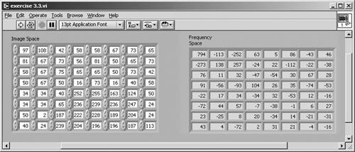
Figure 3.37. Diagram of Exercise 3.3

The inverse 2-D DCT (8 x 8) is defined as

Equation 3.5

 

with k , l = 0, 1, ... , 7, resulting in the original image. An important issue is that the formulas for the DCT and the inverse DCT are more or less the same; this makes it easy for hardware implementation solutions to use specific calculation units.

You can easily find tools on the Internet for the calculation of the DCT coefficients and the inverse DCT; a very good one is at www-mm.informatik.uni-mannheim.de/veranstaltungen/animation/multimedia/2d_dct/, shown in Figure 3.38.

Figure 3.38. DCT and Inverse DCT Calculation

JPEG Coding

You may argue that up to now there has not been any data reduction at all, because the 64 brightness values result in 64 DCT coefficients, and you are right. On the other hand, it is easy to reduce the number of DCT coefficients without losing significant image content.

For example, take a look at the coefficients in Figure 3.35 or Figure 3.36. The most important values, which contain most of the image information, are in the upper-left corner. If coefficients near the lower-right corner are set to 0, a certain degree of compression can be reached. Usually, the coefficient reduction is done by division by a quantization table , which is an 8 x 8 array with certain values for each element.

In the 1980s, the JPEG (Joint Photographic Experts Group) started the development of a standard for the compression of colored photographic images, based on the DCT. Figure 3.39 shows the result for the quantization of the DCT coefficients in our example and the reconstructed image.

Figure 3.39. DCT and Inverse DCT Calculation with JPEG Quantization

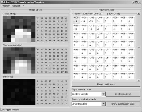
Figure 3.40 shows on its left side the respective JPEG quantization table. The right half of Figure 3.40 shows, that if the resulting coefficients are grouped in a specific order (top left to bottom right), long blocks of consecutive 0s can be found. These blocks are RLE- and Huffman-coded to obtain a compression optimum.

Figure 3.40. JPEG Quantization Table and Coefficient Reading

Discrete Wavelet Transform (DWT)

A significant disadvantage of DCT and JPEG compression is that the DCT coefficients describe not only the local image content but also the content of a wider range, because of the continuous cosine functions. The results are the well-known JPEG blocks (8 x 8 pixels, as we already know) surrounded by strong color or brightness borders.

Another possibility is the use of wavelets instead of cosine functions. The name wavelet comes from "small wave" and means that the signals used in this transformation have only a local impact. Figure 3.41 shows an example from the LabVIEW Signal Processing Toolkit (available as an add-on).

Figure 3.41. 2D Wavelet Transform Example (LabVIEW Signal Processing Toolkit)

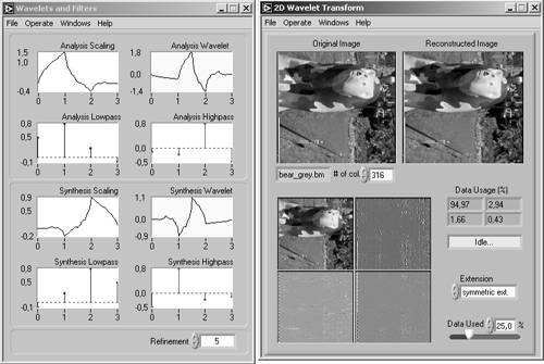
The DWT does the following: it splits the image, by using filters based on wavelets, into two frequency areashigh-pass and low-pass which each contain half of the information and so, if combined, result in an "image" of the original size. This process is repeated. The equations used for this transformation are

Equation 3.6

 

Equation 3.7

 

where l and h are the filter coefficients and p is an integer giving the number of filter applications. w and f are the results of high-pass and low-pass filter application, respectively. The inverse transform is performed by

Equation 3.8

 

JPEG2000 Coding

The JPEG2000 group, starting with its work in 1997, developed the new standard for image compression that uses the DWT, resulting in images with the extension .j2k . After compression with DWT, JPEG2000 uses arithmetic coding instead of Huffman [10] for the coefficients. You can compare the results of JPEG and JPEG2000 by using, for example, a tool from www.aware.com; the results are also evident in Figure 3.42.

[10] Huffman coding is used in JPEG.

Figure 3.42. JPEG2000 Generation Tool (www.aware.com)

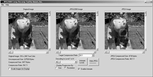
In this example, a section of about 35 x 35 pixels is enlarged in Figure 3.43. The 8 x 8 pixel areas in the JPEG version are clearly visible, whereas the JPEG2000 version shows a significantly better result. Both compressed images were generated with a compression ratio of about 60:1.

Figure 3.43. Comparison of JPEG and JPEG2000 Image Areas

Image Standards