Other Image Sources

This section clarifies that ( especially in the life sciences) image sensors or cameras themselves are not the only possibility for the generation of images. I discuss ultrasound imaging devices, computer tomography and its derivatives, and magnetic resonance imaging (MRI).

Ultrasound Imagers

Ultrasound imaging devices are based on the principle of the different sound impedances of different body tissue classes, resulting in reflection and refraction of the sound waves, similar to the respective optical effects. An ultrasound head is used for the emission as well as for the reception of short sound packets, as shown in Figure 2.36.

Figure 2.36. Principle of Ultrasound A and M Mode [19]

The A mode simply displays the reflections of the tissue boundaries (Figure 2.36). This information plotted over time is called M mode . Figure 2.36 also shows an M mode display in connection with the electrocardiogram (ECG) [19].

For ultrasound "images" to be obtained from the area of interest, it is necessary to move the sound head over a defined region (2D ultrasound or B mode ). Sound heads that perform this movement automatically are called ultrasound scanners . Mechanical scanners, used in the early days of ultrasound imaging devices, are nowadays replaced by electronic scanning heads. The example shown in Figure 2.37 uses a curved array of ultrasound elements, which are activated in groups and electronically shifted in the desired direction.

Figure 2.37. Curved Array Ultrasound Head and Corresponding Image

Some more information about sound reflection and refraction: Like the corresponding optical effects, the reflection of sound waves at tissue boundaries with different sound impedance is described by the reflection factor R :

Equation 2.22

with Z i as the sound impedance of the respective area and the transmission factor T :

Equation 2.23

This is why a special ultrasound transmission gel has to be applied to the sound head before it is attached to the skin; otherwise , almost all of the sound energy would be reflected. Table 2.6 shows examples for the reflection factor R at some special tissue boundaries.

Table 2.6. Typical Values of the US Reflection Factor R

from/to:	Fat	Muscle	Liver	Blood	Bone
Water:	0.047	0.020	0.035	0.007	0.570
Fat:		0.067	0.049	0.047	0.610
Muscle:			0.015	0.020	0.560
Liver:				0.028	0.550
Blood:					0.570

Computed Tomography

The principle of computed tomography (CT) is based on x-ray imaging, which makes use of the characteristic attenuation of x-rays by different tissue types. X-ray imaging generates only a single image, showing a simple projection of the interesting region. CT, on the other hand, can display cross sections of the body, so the imaging device has to "shoot" a large number of attenuation profiles from different positions around the body. An important issue is the reconstruction of the resulting image.

Looking at the simplest case of a homogeneous object of interest, [8] we see that the intensity I of the detected radiation decreases exponentially with the object width d and is therefore given by

[8] This case also includes radiation of one single frequency.

Equation 2.24

 

whereas the attenuation P is defined by the product of the attenuation coefficient m and the object width d :

Equation 2.25

 

finally, the attenuation coefficient itself is therefore

Equation 2.26

 

CT Device Generations

Computed tomography devices are usually classified in "generations," as shown in Figure 2.38:

Figure 2.38. CT Device Generations 1 to 4 [20]

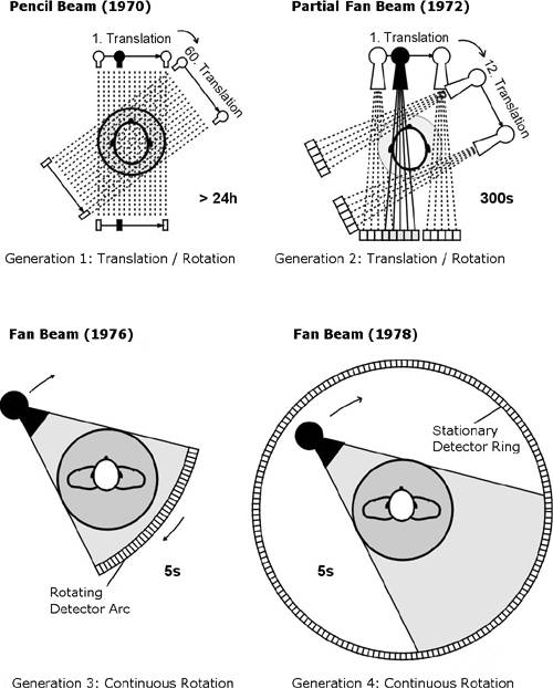
• Scanning by use of a single "pencil beam"; the beam is shifted and rotated (generation 1).
• The needle beam is replaced by a "partial fan beam," which again is shifted and rotated (generation 2).
• A fan beam, which is only rotated in connection with the detector array, is able to scan the entire angle area (generation 3).
• Now only the fan beam rotates, whereas the detector array is fixed and covers the entire area in ring form (generation 4).

CT Image Calculation and Back Projection

As you can imagine, it is not easy to obtain the resulting image (the spatial information), because each beam [9] delivers the total attenuation value of its route; we defined the resulting intensity I in Eq. (2.24) for the simple case of a homogeneous object. In most cases, this will not be true; Eq. (2.24) therefore becomes

[9] Here, we are considering a CT device of generation 1.

Equation 2.27

 

with m i as the attenuation coefficient in a specific area and d i as the respective length of this area, for the intensity I in a certain direction.

Figure 2.39. Simple Calculation of a CT Image [20]

Special algorithms are necessary for computation of the original values m i of a certain area. The following solutions can be used:

1. As shown in Figure 2.39, the simplest method is to solve the equation system consisting of N 2 variables resulting from the intensity values of the different directions. Figure 2.39 shows this principle for 2 x 2 and 3 x 3 CT images.
2. It is easy to imagine that method 1 will lead to huge equation arrays and a much too high calculation amount if the pixel number of the image increases . Therefore, the equation systems of existing systems must be solved in an iterative way. An example of this method is described in Exercise 2.5.
3. Today, the method of filtered back projection is usually used. Normal back projection (summation of the projections in each direction) would lead to unfocused images; therefore, the projections are combined with a convolution function to correct the focus on the edges.

A good example, which illustrates the method of back projection, can be found at the National Instruments web page www.ni.com; just go to "Developer Zone," search for "tomography," and download the LabVIEW library Tomography.llb (see Figure 2.40).

Figure 2.40. Tomography Simulation (National Instruments Example)

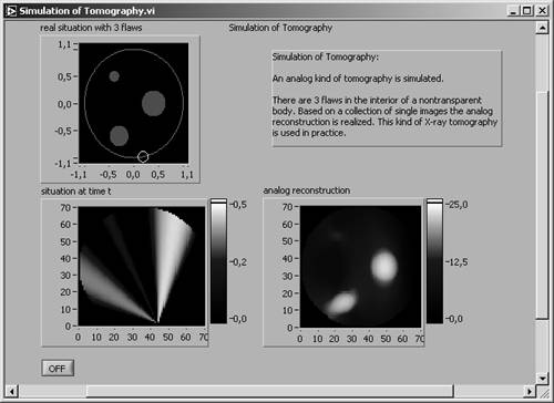
Figure 2.41. Iterative Calculation of a CT Image

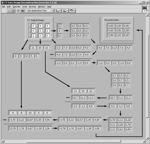
Exercise 2.5: Iterative Calculation of a CT Image.

Try to make the iterative calculation (method 2) in a LabVIEW VI (front panel shown in Figure 2.41). Here, the intensity values of four directions are used, starting with the one to the right. The first estimation is based on the equal distribution of the intensity values over the entire lines. The values of the next direction (bottom right) are calculated and compared to the values of the original image. The difference of these results is applied to the first estimation, resulting in the second estimation, and so on.

As you will find out, the values already are quite close to the original values. You can get the values closer to the original if you run the previously described steps again with the new values. After a third run, the differences will be too small to notice.

 

Single Photon Emission Computed Tomography (SPECT)

This method is quite similar to computer tomography with respect to image generation. The main difference is that the total emitted gamma radiation, not an attenuation coefficient, of a specific direction is measured. Therefore, the same imaging techniques (usually filtered back projection) can be used.

Positron Emission Tomography (PET)

PET is based on the detection of gamma quants that result from the collision of an electron with a positron. To make this possible, interesting molecules have to be marked before imaging with a positron radiator; we do not discuss this process here.

In general, for PET images the same image generation processes that have been described above can be used; here, the main difference is that the machine cannot decide ahead of time which direction is to be measured. However, it is possible to afterwards assign specific events to the appropriate projection directions.

Magnetic Resonance Imaging

Magnetic resonance imaging (MRI; sometimes NMRI for nuclear MRI) uses a special property of particular atoms and especially their nuclei; this property, called spin , is related to the number of protons and neutrons. The spin is represented by the symbol I and always occurs in multiples of 1/2. For example, the nucleus of 1 H has a spin of I = 1/2 and the nucleus of 17 O a spin of I = 5/2.

In Figure 2.42, the spin of a nucleus is visualized by an arrow (up or down), which indicates that the nuclei are "rotating" around the arrow axis clockwise or counterclockwise, respectively. If an external magnetic field B is applied, the (usually unoriented) spins may align parallel or anti-parallel to this field.

Figure 2.42. Separation of Energy Levels According to Spin Directions

The energy necessary for the transition from the parallel to the anti-parallel state depends on the value of the external magnetic field B and is given as

Equation 2.28

 

with h as Planck's constant and g as the intrinsic gyromagnetic ratio. Integrated in Eq. (2.28) is the Larmor equation

Equation 2.29

 

which indicates that the frequency related to the nuclei [10] depends on the value of the external magnetic field.

[10] This is the so-called precession frequency.

If the energy of Eq. (2.28) is applied to some nuclei, a large number of them are raised from their state of lower energy to the state of higher energy. After a certain time, the nuclei return to their original state, emitting the energy D E .

Figure 2.43. Relaxation Times T 1 and T 2

The magnetization M can be split into a component M xy residing in the xy plane and a component M z in z direction. After excitation of the nuclei with a certain frequency pulse, both magnetization components follow the equations

Equation 2.30

 

and

Equation 2.31

 

(see also Figure 2.43) with the specific relaxation times T 1 and T 2 . Table 2.7 shows some different values for some important tissue types.

If the Larmor equation (2.29) can be modified to

Equation 2.32

 

with w ( r i ) as the frequency of a nucleus at the location r i and describing the gradient location-dependent amplitude and direction, the location r i of the nucleus can be specified. The final imaging techniques are quite similar to those used in computer tomography but offer a number of additional possibilities:

Table 2.7. Typical Values of Relaxation Times T 1 and T 2 at 1 Tesla

Tissue Type	Relaxation Time T 1	Relaxation Time T 2
Muscle:	730 ± 130 ms	47 ± 13 ms
Heart:	750 ± 120 ms	57 ± 16 ms
Liver:	420 ± 90 ms	43 ± 14 ms
Kidney:	590 ± 160 ms	58 ± 24 ms
Spleen:	680 ± 190 ms	62 ± 27 ms
Fat:	240 ± 70 ms	84 ± 36 ms

• It is possible to distinguish more precisely between tissue types, compared with methods , such as CT, that use only the attenuation coefficient. Different tissue types can have identical attenuation coefficients but totally different relaxation times T 1 and T 2 because of their different chemical structure.
• Another possibility is to scale the gray scales of the image according to the respective relaxation times. As can be seen in Table 2.7, T 1 and T 2 do not have a direct relationship. Figure 2.44 shows an example for a T 1 and a T 2 weighted image.

Figure 2.44. MRI Images: Based on T 1 (left) and T 2 (right) of a Knee Joint

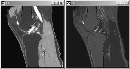
Image Distribution