Frequency Filtering

If we follow this idea further, we should be able to describe the entire image by a set of frequencies. In electrical engineering, every periodic waveform can be described by a set of sine and cosine functions, according to the Fourier transform and as shown in Figure 4.32.

Figure 4.32. Waveform Spectrum

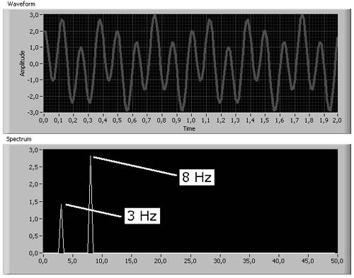
Here, the resulting waveform consists of two pure sine waveforms, one with f 1 = 3 Hz and one with f 2 = 8 Hz, which is clearly visible in the frequency spectrum, but not in the waveform window at the top. A rectangular waveform, on the other hand, shows sharp edges and thus contains much higher frequencies as well.

Coming back to images, the Fourier transform is described by

Equation 4.18

with s ( x,y ) as the pixel intensities. Try the following exercise.

Exercise 4.8: Frequency Representation of Images.

Create a frequency representation of our bear image by using the function IMAQ FFT . You can switch between two display modes, using IMAQ ComplexFlipFrequency (both functions are described later). Note that the image type of the frequency image has to be set to Complex (see Figures 4.33 and 4.34).

 

Figure 4.33. FFT Spectrum of an Image

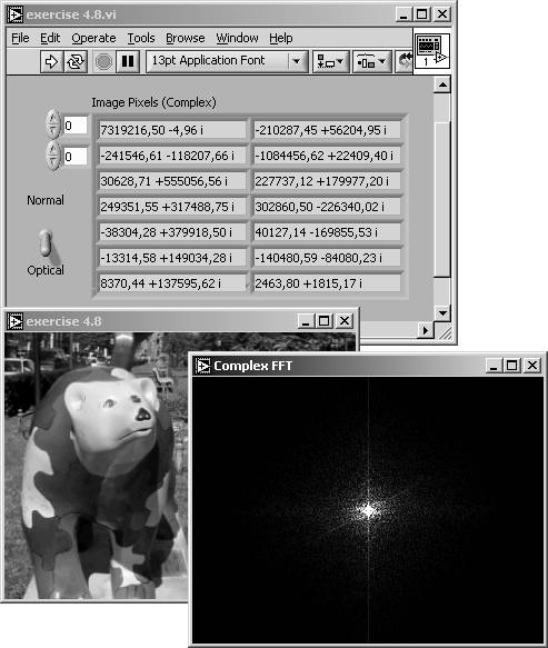
Figure 4.34. FFT Spectrum of an Image

The exponential function of Eq. (4.18) can also be written as

Equation 4.19

 

and that is why the entire set of pixel intensities can be described by a sum of sine and cosine functions but the result is complex. [4]

[4] On the other hand, the complex format makes it easier to display the results in a two-dimensional image.

IMAQ Vision uses a slightly different function for the calculation of the spectral image, the fast Fourier transform (FFT). The FFT is more efficient than the Fourier transform and can be described by

Equation 4.20

 

where n and m are the numbers of pixels in x and y direction, respectively.

Figure 4.35 shows another important issue: the difference between standard display of the fast Fourier transform and the optical display . The standard display groups high frequencies in the middle of the FFT image, whereas low frequencies are located in the four corners (left image in Figure 4.35). The optical display behaves conversely: Low frequencies are grouped in the middle and high frequencies are located in the corners. [5]

[5] Note a mistake in IMAQ Vision's help file: IMAQ FFT generates output in optical display, not in standard.

Figure 4.35. FFT Spectrum (Standard and Optical Display)

FFT Filtering: Truncate

If we have the entire frequency information of an image, we can easily remove or attenuate certain frequency ranges. The simplest way to do this is to use the filtering function IMAQ ComplexTruncate . You can modify Exercise 4.8 to do this.

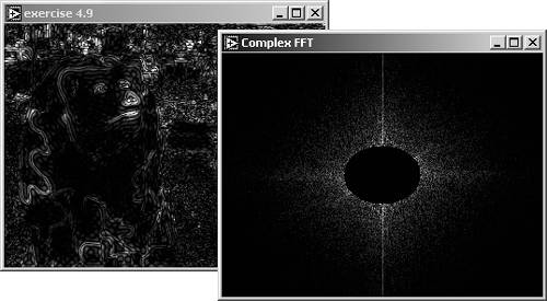
Exercise 4.9: Truncation Filtering.

Add the function IMAQ ComplexTruncate to Exercise 4.8 and also add the necessary controls (see Figures 4.36 and 4.37). The control called Truncation Frequencies specifies the frequency percentage below which (high pass) or above which (low pass) the frequency amplitudes are set to 0.

In addition, use IMAQ InverseFFT to recalculate the image, using only the remaining frequencies. Figure 4.36 shows the result of a low-pass truncation filter; Figure 4.38, the result of a high-pass truncation filter.

 

Figure 4.36. FFT Low-Pass Filter

Figure 4.37. Diagram of Exercise 4.9

Figure 4.38. FFT High-Pass Filter

The inverse fast Fourier transform (FFT) used in Exercise 4.9 and in the function IMAQ InverseFFT is calculated as follows :

Equation 4.21

 

FFT Filtering: Attenuate

An attenuation filter applies a linear attenuation to the full frequency range. In a low-pass attenuation filter, each frequency f from f to f max is multiplied by a coefficient C , which is a function of f according to

Equation 4.22

 

It is easy to modify Exercise 4.9 to a VI that performs attenuation filtering.

Exercise 4.10: Attenuation Filtering.

Replace the IMAQ Vision function IMAQ Complex Truncate with IMAQ ComplexAttenuate and watch the results (see Figure 4.39). Note that the high-pass setting obviously returns a black image; is that true?

 

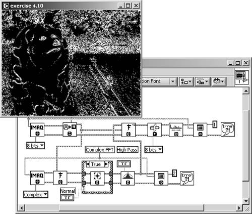
The formula for the coefficient C in a high-pass attenuation filter is

Equation 4.23

 

which means that only high frequencies are multiplied by a significantly high coefficient C ( f ). Therefore, the high-pass result of Exercise 4.10 (Figure 4.40) contains a number of frequencies that are not yet visible. You may insert the LuT function IMAQ Equalize to make them visible (do not forget to cast the image to 8 bits).

Figure 4.39. FFT Low-Pass Attenuation Filter

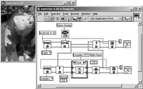
Figure 4.40. FFT High-Pass Attenuation Result

Morphology Functions