Appendix E EOQ vs. Kanban

Overview

A kanban model can sometimes lead you to a solution that requires an unrealistic number of changeovers. Since kanban formulation logic only considers time and does not consider the cost of changeovers, the final calculation can result in a solution that minimizes run size and inventory levels but schedules a large number of changeovers. An EOQ model can be utilized to give you a different solution that can be used as a sanity check on the kanban solution. EOQ models seek to find an optimum solution by determining the mathematical minimum total cost, taking into account holding cost and changeover costs. Although some companies apply the EOQ model directly, its logic is also used in some MRP/ERP systems. There are significant differences in the solutions generated by each method (EOQ versus kanban).

Kanban seeks to minimize inventory by minimizing the replenishment interval, which essentially drives you toward increasingly small lot sizes. This means that as you improve efficiency (for example, through reduced changeover times or decreased downtime), the kanban model will utilize this extra time to reduce the replenishment interval (and thus increase the number of changeovers.)

The EOQ model, however, seeks only to minimize cost. It will use any improvement in efficiency to reduce total system costs. Thus, as you increase efficiency, the optimal solutions given by the two models will change.

EOQ Model

The goal of the EOQ model is to determine the optimum procedure for producing a given quantity of product that minimizes holding and set-up costs while preventing stock outs. In our simplified example, we will set up a two-day safety stock that provides us with a 100 percent certainty that there will not be any stock outs (wouldn't it be nice if it were that easy in real life?). The model assumes a rotational cycle. This means that it assumes that every product is only set up once during the production cycle, similar to the replenishment cycle used in kanban calculations. As you will see below, the EOQ model's focus on cost minimization can create unrealistic solutions. We will compare the results of the EOQ model with the kanban model in an analysis of a fictional company that manufactures plastic components on one machine.

In this analysis, our company makes nine different products, some in multiple lengths. In this model, we plan for a two-day safety stock to avoid stock outs (the cost of stock outs is zero). We also input line speeds and changeover time (changeover time for length changes only is zero).

This is a simple model to demonstrate how EOQ models work. There are many different variations that can be incorporated into this model to fit real-world situations. In this simple model, we are seeking the minimum total cost; balancing holding costs with setup (or ordering) costs. Set-up costs (f) are calculated as the cost of a machine set-up, including both the scrap generated and the labor required to perform the set-up. Holding costs (h) are the cost of holding inventory, which includes the value of the capital tied up in inventory (calculated as the firm's cost of capital, which in this case we will assume to be 12 percent). If there is an alternate revenue-producing use of floor space occupied by the inventory, then this also needs to be included in the holding costs. For our example, we assume this is not the case.

Under our EOQ model, the minimum cost (and thus the optimum lot size) for a lot size equal to q* occurs where it is possible to show that q* = ˆ 2fd/h, where d equals the demand rate on an annual basis.

q* = ˆ (2fd/h)

In the analysis below, we examine the solutions offered by a kanban model and an EOQ model. We also examine the impacts of productivity changes on the solutions that each system generates. As you will see, the two models offer very different solutions. The EOQ model drives toward a solution with large inventories in an attempt to minimize total system costs. The kanban system drives to a solution with ever-shrinking lot sizes. In analyzing the different solutions, keep in mind that many of the benefits of the kanban system are difficult to quantify (more flexibility, reduced quality exposure, and employee empowerment). By its nature, the EOQ model seeks to minimize all quantifiable costs. Thus, the EOQ model will generally provide a solution that yields a lower quantifiable total cost than a kanban system. However, also keep in mind that both models are strongly influenced by the cost assumptions used. The value of floor space and the cost of capital, for example, both have a large impact on the EOQ solution.

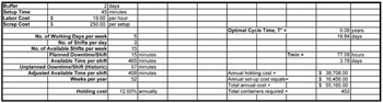
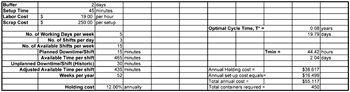
For our kanban model, we created a spreadsheet to calculate the number of containers used to control production for individual products. Based on average daily requirements, production losses and secondary process losses, the spreadsheet calculates the adjusted daily requirement (the quantity of product to be produced to meet the average demand from the customer). Daily run-time requirements are then calculated by multiplying the adjusted daily requirement by the production cycle time required per piece. These run times are then summed to calculate the daily run-time requirement.

Available production time, daily run-time requirements, and total set-up time are used by the kanban spreadsheet to determine the production cycle. Available time is calculated by subtracting downtime, both planned and unplanned , from the total scheduled hours. Using the total run-time requirement and the available time, time available for set-ups is calculated.

Total Available - Time Total Run Time = Available Set-up Time

If this number is less than zero, there is no feasible answer and there is a shortage of capacity on the particular production line. If the number is positive, the total set-up time for the production cycle is divided by the available set-up time to determine the replenishment interval.

Days per Cycle = Total Set-up Time / Available Set-up Time

Based on the capacity of the containers for individual parts , the appropriate number of containers is calculated to match the buffer size of two days plus the production run quantity. Production run quantities of each part are calculated by multiplying the production cycle by the adjusted daily requirements. The production quantity plus buffer quantity divided by part capacity per container determines the total number of containers required to control production.

What advantages does this solution offer? The system minimizes the production cycle and gives the benefit of speed and flexibility. If demand is volatile and requirements for an individual part change, you can respond quickly, reducing the reliance on forecasts and the need for expediters to help adjust to schedule variations. This system also minimizes inventory and reduces the risk of obsolescence. These lower inventory levels reduce quality risks, since production defects may be detected earlier with fewer parts at risk. The use of the kanban signals also allows operators to schedule their own production activities, reducing the need for a large production control department.

The Effect of Productivity Improvements

Let's begin to examine the effects of productivity improvements on the different models. Lets assume a SMED program is launched that will reduce set-up time from 45 minutes to 23 minutes. Additionally, scrap costs incurred during set-ups are targeted for reductions from $100 to $75 per set-up. As reductions in set-up time are made, the kanban model drives closer to the theoretical optimum lot size of one piece. Unfortunately, it does this without consideration of changeover costs. If set-up costs are not reduced proportionally to set-up time reductions, the kanban model actually makes recommendations that increase costs by increasing the total set-up costs. The only consideration is time, with available capacity being fully utilized with additional set-ups. With the current planning model, the targeted SMED results will increase operating costs.

Let's also assume a TPM program is launched that reduces unscheduled downtime for the production lines. Current historical averages for downtime are 15 minutes of planned downtime per shift and 57 minutes of unplanned downtime. Unplanned downtime has been targeted, with a goal of 30 minutes of unplanned downtime per shift. As these efforts are made to increase available production time, the kanban system makes further reductions in cycle time (see Table E-1).

Table E-1: Kanban cycle time.

	Cycle Time Days	Annual Holding Costs	Annual Setup Costs	Total Costs
Current	3.78	$5,418	$ 86,430	$ 91,847
After SMED	1.93	$3,663	$112,160	$115,823
After downtime reduction	2.04	$4,506	$159,906	$164,412
Nirvana	1.04	$3,663	$207,510	$211,173

EOQ Model Basic Cycle

The EOQ model optimizes the production system based on total holding and changeover costs. Unlike the kanban, the EOQ model is not concerned specifically with time unless a dollar value is attached to the time. Improvements in available time only shorten the production cycle time by the improvement. So downtime reduction efforts only cause minor changes in the calculated cycle. Reductions in set-up costs have a direct impact on the calculated cycle; it becomes more economical to change more frequently, which also reduces average inventory levels and associated holding costs. But these changes are a result of total set-up costs, not just the time required for set-ups. Since our fictional company incurs significant cost in scrap material for each set-up, this is critical.

EOQ Model Rotation Cycle

Table E-2 shows the calculated production cycles before any productivity improvements. Several products in our example share common set-ups, eliminating the set-up costs. These products are sequenced to avoid these unnecessary set-ups. This same sequence was also used in the kanban schedule. Total costs are significantly lower than the kanban system, but at higher inventory levels with longer production cycles. In efforts to achieve speed and low inventory levels, it appears as though the kanban model will incur significant additional costs. Remember, many of the benefits of the kanban system are difficult to quantify, so use judgment when viewing calculations that show that the kanban solution drives up costs.

As improvement efforts pay off in reductions to set-up costs, the total cost of the production system shows improvement. However, the EOQ model calculates the reduction in cycle time based on the reduction of the total cost of changeovers, not just the reduction in time required. The improvements in equipment uptime, however, do not have a significant impact on the total cost (see Table E-3 for the production cycle after the implementation of SMED and TPM).

Production Constraints

Space requirements for inventory may become a constraint for the EOQ solution. Assume a container size of 3' x 6' (18 square feet). The EOQ solution requires an increase from 126 containers to 452, but reduces identified costs from $91,847 to $55,165. Assuming 75 percent utilization of floor space, this gives an increase in floor space requirements of 7,824 square feet. Depending on the available floor space in the plant, this may not be feasible . Again, if there were an identified alternative use of the floor space that would produce revenue, then this cost would need to be added to the model. Table E-4 shows the cycle times and total costs of the EPQ solutions.

Table E-4

Cycle Time (in Days)	Annual Holding Costs	Annual Setup Costs	Total Costs
Current	19.8	$38,709	$16,457	$55,166
After SMED	16.2	$32,093	$13,403	$45,496
After Downtime	19.8	$38,617	$16,499	$55,117
Nirvana	16.1	$32,018	$13,437	$45,455

Although the EOQ model seems to give a lower cost solution, you need to use caution when comparing the models. The EOQ model places no value on reductions in inventory (except for the minor reduction in holding costs), and no value on quality improvements, increased flexibility, or employee empowerment. With the kanban model, the value of the intangible benefits of speed, flexibility, and very low inventory levels need to be considered . Plotting the costs of scheduling options versus total cost as shown in Figure E-1 should be done during each planning cycle. This provides an easy method to evaluate the cost impact of planning decisions. Also note that as changeover time and cost approaches zero, both models will give very similar solutions.

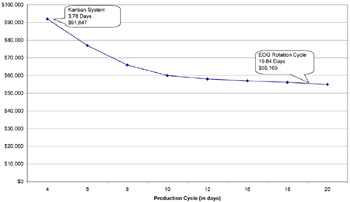
Figure E-1: Total Cost

The EOQ model also highlights the need to assess total cost when determining kanban quantities. Smaller batch sizes may produce larger total costs. Keep this thought in mind as you reduce kanban quantities .