Morphology Functions

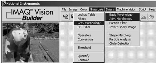
If you search IMAQ Vision Builder's menus for morphology functions, you will find two different types (Figure 4.41):

• Basic and Advanced Morphology in the Binary menu;
• Gray Morphology in the Grayscale menu.

Figure 4.41. Morphology Functions in IMAQ Vision Builder

Basically, morphology operations change the structure of particles in an image. Therefore, we have to define the meaning of "particle"; this is easy for a binary image: Particles are regions in which the pixel value is 1. The rest of the image (pixel value 0) is called background . [6]

[6] Remember that a binary image consists only of two different pixel values: 0 and 1.

That is why we first learn about binary morphology functions; gray-level morphology is discussed later in this section.

Thresholding

First of all, we have to convert the gray-scaled images we used in previous exercises into binary images. The function that performs this operation is called thresholding . Figure 4.42 shows this process, using IMAQ Vision Builder: two gray-level values, adjusted by the black and the white triangle, specify a region of values within which the pixel value is set to 1; all other levels are set to 0.

Figure 4.42. Thresholding with IMAQ Vision Builder

Figure 4.43 shows the result. Here and in the Vision Builder, pixels with value 1 are marked red. In reality, the image is binary, that is, containing only pixel values 0 and 1.

Figure 4.43. Result of Thresholding Operation

Next , we try thresholding directly in LabVIEW and IMAQ Vision.

Exercise 4.11: Thresholded Image.

Use the function IMAQ Threshold to obtain a binary image. In this case, use a While loop so that the threshold level can be adjusted easily. Note that you have to specify a binary palette with the function IMAQ GetPalette for the thresholded image. Compare your results to Figures 4.44 and 4.45.

 

Figure 4.44. Thresholding with IMAQ Vision

Figure 4.45. Diagram of Exercise 4.11

IMAQ Vision also contains some predefined regions for areas with pixel values equal to 1; they are classified with the following names :

• Clustering
• Entropy
• Metric
• Moments
• Interclass Variance

All of these functions are based on statistical methods . Clustering , for example, is the only method out of these five that allows the separation of the image into multiple regions of a certain gray level if the method is applied sequentially. [7] All other methods are described in [4]; Exercise 4.12 shows you how to use them and how to obtain the lower value of the threshold region (when these methods are used, the upper value is always set to 255):

[7] Sequential clustering is also known as multiclass thresholding [4].

Exercise 4.12: Auto Thresholding.

Replace the control for adjusting the threshold level in Exercise 4.11 by the function IMAQ AutoBThreshold , which returns the respective threshold value, depending on the image, of course, and the selected statistical method. See Figures 4.46 and 4.47.

 

Figure 4.46. Predefined Thresholding Functions

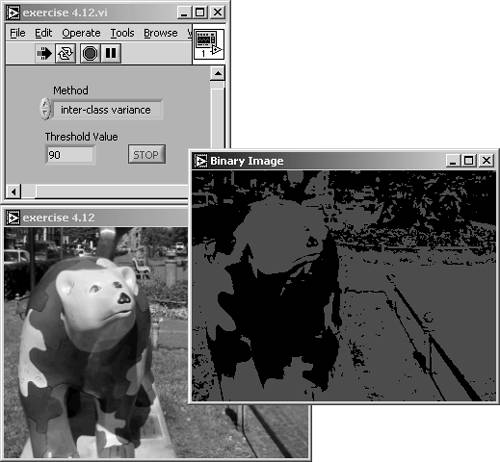
Figure 4.47. Diagram of Exercise 4.12

Reference [4] also gives the good advice that sometimes it makes sense to invert your image before applying one of those threshold methods, to get more useful results.

An interesting method for the separation of objects from the background is possible if you have a reference image of the background only. By calculating the difference image of these two and then applying a threshold function, you will get results of a much higher quality. You can read more about difference images in the application section of Chapter 5.

IMAQ Vision also contains a function ” IMAQ MultiThreshold ”that allows you to define multiple threshold regions to an image. By the way, you can also apply threshold regions to special planes of color images, for example, the hue plane. You can also find an interesting application that uses this method in Chapter 5.

What about direct thresholding of color images? If you use the function IMAQ ColorThreshold , you can directly apply threshold values to color images; either to the red, green, and blue plane (RGB color model) or to the hue, saturation, and luminance plane (HSL color model).

A final remark: Because we usually display our images on a computer screen, our binary images cannot have only pixel values of 0 and 1; in the 8-bit gray-scale set of our monitor, we would see no difference between them. Therefore, all image processing and analysis software, including IMAQ Vision, displays them with gray-level values of 0 and 255, respectively.

Binary Morphology

As explained above, morphology functions change the structure of objects (often called particles ) of a (usually binary) image. Therefore, we have to define what the term structure (or shape ) means.

We always talk about images, which use pixels as their smallest element with certain properties. Objects or particles are coherent groups of pixels with the same properties ( especially pixel value or pixel value range). The shape or structure of an object can be changed if pixels are added to or removed from the border (the area where pixel values change) of the object.

To calculate new pixel values, structuring elements are used: the group of pixels surrounding the pixel to be calculated. Figure 4.48 shows some examples of the elements defined below:

• The shape of the structuring element is either rectangular (square; left and center examples) or hexagonal (example on the right).
• The connectivity defines whether four or all eight surrounding pixels are used to calculate the new center pixel value. [8]

  [8] In the case of a 3 x 3 structuring element.

Figure 4.48. Examples of Structuring Elements

The symbols at the top of Figure 4.48 are used by IMAQ Vision Builder to indicate or to set the shape and the connectivity of the structuring element. A 1 in a pixel means that this pixel value is used for the calculation of the new center pixel value, according to

Equation 4.24

 

for connectivity = 4 and

Equation 4.25

 

for connectivity = 8.

It is also possible to define other (bigger) structuring elements than the 3 x 3 examples of Figure 4.48. In IMAQ Vision Builder, 5 x 5 and 7 x 7 are also possible. Note that the procedure is quite similar to the filtering methods we discussed in a previous section.

In IMAQ Vision Builder, you can change the shape of the structuring element by simply clicking on the small black squares in the control (see Figure 4.49).

Figure 4.49. Configuring the Structuring Element in IMAQ Vision Builder

In our following examples and exercises we use a thresholded binary image, resulting from our gray-scaled bear image, by applying the entropy threshold function (or you can use manual threshold; set upper level to 255 and lower level to 136). The resulting image (Figure 4.50) contains a sufficient number of particles in the background, so the following functions have a clearly visible effect.

Erosion and Dilation

These two functions are fundamental for almost all morphology operations. Erosion is a function that basically removes (sets the value to 0) pixels from the border of particles or objects. If particles are very small, they may be removed totally.

The algorithm is quite easy if we consider the structuring element, centered on the pixel (value) s : If the value of at least one pixel of the structuring element is equal to 0 (which means that the structuring element is located at the border of an object), s is set to 0, else s is set to 1 (Remember that we only consider pixels masked with 1 in the structuring element) [4].

We can test all relevant morphology functions in Exercise 4.13.

Exercise 4.13: Morphology Functions.

Create a VI that displays the results of the most common binary morphology functions, using the IMAQ Vision function IMAQ Morphology . Make the structuring element adjustable with a 3 x 3 array control. Compare your results to Figure 4.50, which also shows the result of an erosion, and Figure 4.51.

Note that some small particles in the background have disappeared; also note that the big particles are smaller than in the original image. Try different structuring elements by changing some of the array elements and watch the results.

 

Figure 4.50. Morphology Functions: Erosion

Figure 4.51. Diagram of Exercise 4.13

A special notation for morphology operations can be found in [13], which shows the structure of concatenated functions very clearly. If I is an image and M is the structuring element (mask), the erosion (operator ) is defined as

Equation 4.26

 

where I a indicates a basic shift operation in direction of the element a of M . I “a would indicate the reverse shift operation [13].

A dilation adds pixels (sets their values to 1) to the border of particles or objects. According to [13], the dilation (operator ) is defined as

Equation 4.27

 

Again, the structuring element is centered on the pixel (value) s : If the value of at least one pixel of the structuring element is equal to 1, s is set to 1, else s is set to 0 [13].

Figure 4.52 shows the result of a simple dilation. Note that some "holes" in objects (the bear's eyes for example) are closed or nearly closed; very small objects get bigger. You can find more information about the impact of different structuring elements in [4].

Figure 4.52. Morphology: Dilation Result

Opening and Closing

Opening and closing are functions that combine erosion and dilation functions. The opening function is defined as an erosion followed by a dilation using the same structuring element. Mathematically, the opening function can be described by

Equation 4.28

 

or, using the operator ,

Equation 4.29

 

Figure 4.53 shows the result of an opening function. It is easy to see that objects of the original image are not significantly changed by opening; however, small particles are removed. The reason for this behavior is that borders, which are removed by the erosion, are restored by the dilation function. Naturally, if a particle is so small that it is removed totally by the erosion, it will not be restored.

Figure 4.53. Morphology: Opening Result

The result of a closing function is shown in Figure 4.54. The closing function is defined as a dilation followed by an erosion using the same structuring element:

Figure 4.54. Morphology: Closing Result

Equation 4.30

 

or, using the operator ,

Equation 4.31

 

Again, objects of the original image are not significantly changed. Complementarily to the opening function, small holes in particles can be closed.

Both opening and closing functions use the duality of erosion and dilation operations. The proof for this duality can be found in [13].

Proper Opening and Proper Closing

IMAQ Vision provides two additional functions called proper opening and proper closing. Proper opening is defined as a combination of two opening functions and one closing function combined with the original image:

Equation 4.32

 

or

Equation 4.33

 

As Figure 4.55 shows, the proper opening function leads to a smoothing of the borders of particles. Similarly to the opening function, small particles can be removed.

Figure 4.55. Morphology: Proper Opening Result

Proper closing is the combination of two closing functions combined with one opening function and the original image:

Equation 4.34

 

or

Equation 4.35

 

Proper closing smooths the contour of holes if they are big enough so that they will not be closed. Figure 4.56 shows that there is only a little difference between the original image and the proper closing result.

Figure 4.56. Morphology: Proper Closing Result

Hit- Miss Function

This function is the first simple approach to pattern matching techniques. In an image, each pixel that has exactly the neighborhood defined in the structuring element (mask) is kept; all others are removed. In other words: If the value of each surrounding pixel is identical to the value of the structuring element, the center pixel s is set to 1; else s is set to 0.

The hit-miss function typically produces totally different results, depending on the structuring element. For example, Figure 4.57 shows the result of the hit-miss function with the structuring element All pixels in the inner area of objects match M ; therefore, this function is quite similar to an erosion function.

Figure 4.57. Hit-Miss Result with Structuring Element That Is All 1s

Figure 4.58 shows the result when the structuring element is used. This mask extracts pixels that have no other pixels in their 8-connectivity neighborhood.

Figure 4.58. Hit-Miss Result with Structuring Element That Is All 0s

It is easy to imagine that the hit-miss function can be used for a number of matching operations, depending on the shape of the structuring element. For example, a more complex mask, like will return no pixels at all, because none match this mask.

More mathematic details can be found in [13]; we use the operator for the hit-miss function: [9]

[9] Davies [13] uses a different one; I prefer because it reminds me of the pixel separation in Figure 4.58.

Equation 4.36

 

Gradient Functions

The gradient functions provide information about pixels eliminated by an erosion or added by a dilation. The inner gradient (or internal edge ) function subtracts the result of an erosion from the original image, so the pixels that are removed by the erosion remain in the resulting image (see Figure 4.59 for the results):

Equation 4.37

 

Figure 4.59. Inner Gradient (Internal Edge) Result

The outer gradient (or external edge ) function subtracts the original image from a dilation result. Figure 4.60 shows that only the pixels that are added by the dilation remain in the resulting image:

Equation 4.38

 

Figure 4.60. Outer Gradient (External Edge) Result

Finally, the gradient function adds the results of the inner and outer gradient functions (see Figure 4.61 for the result):

Equation 4.39

 

Figure 4.61. Morphology: Gradient Result

Thinning and Thickening

These two functions use the result of the hit-miss function. The thinning function subtracts the hit-miss result of an image from the image itself:

Equation 4.40

 

which means that certain pixels that match the mask M are eliminated. Similarly to the hit-miss function itself, the result depends strongly on the structuring element. [10] Figure 4.62 shows the result for the structuring element

[10] According to [4], the thinning function does not provide appropriate results if s = 0. On the other hand, the thickening function does not work if s = 1.

Figure 4.62. Morphology: Thinning Result

The thickening function adds the hit-miss result of an image to the image itself (pixels matching the mask M are added to the original image):

Equation 4.41

 

Figure 4.63 shows the result of a thickening operation with the structuring element Both functions can be used to smooth the border of objects and to eliminate single pixels (thinning) or small holes (thickening).

Figure 4.63. Morphology: Thickening Result

Auto-Median Function

Finally, the auto-median function generates simpler particles with fewer details by using a sequence of opening and closing functions, according to

Equation 4.42

 

or, using the operator ,

Equation 4.43

 

Figure 4.64 shows the result of applying the auto-median function to our binary bear image.

Figure 4.64. Morphology: Auto-Median Result

Particle Filtering

For the next functions, which can be found under the Adv. Morphology menu in IMAQ Vision Builder, we have to slightly modify our Exercise 4.13 because the IMAQ Morphology function does not provide them.

The remove particle function detects all particles that are resistant to a certain number of erosions. These particles can be removed (similarly to the function of a low-pass filter), or these particles are kept and all others are removed (similarly to the function of a high-pass filter).

Exercise 4.14: Removing Particles.

Replace the function IMAQ Morphology in Exercise 4.13 with IMAQ RemoveParticle . Provide controls for setting the shape of the structuring element (square or hexagonal), the connectivity (4 or 8), and the specification of low-pass or high-pass functionality. See Figure 4.65, which also shows the result of a low-pass filtering, and Figure 4.66.

 

Figure 4.65. Remove Particle: Low Pass

Figure 4.66. Diagram of Exercise 4.14

Figure 4.67 shows the result of high-pass filtering with the same settings. It is evident that the sum of both result images would lead again to the original image.

Figure 4.67. Remove Particle: High Pass

The next function, IMAQ RejectBorder , is quite simple: The function removes particles touching the border of the image. The reason for this is simple as well: Particles that touch the border of an image may have been truncated by the choice of the image size. In case of further particle analysis, they would lead to unreliable results.

Exercise 4.15: Rejecting Border Particles.

Replace the function IMAQ Morphology in Exercise 4.13 or IMAQ RemoveParticle in Exercise 4.14 by IMAQ RejectBorder . The only necessary control is for connectivity (4 or 8). See Figures 4.68 and 4.69.

 

Figure 4.68. Particles Touching the Border Are Removed

Figure 4.69. Diagram of Exercise 4.15

The next function ” IMAQ ParticleFilter ”is much more complex and much more powerful. Using this function, you can filter all particles of an image according to a large number of criteria. Similarly to the previous functions, the particles matching the criteria can be kept or removed, respectively.

Exercise 4.16: Particle Filtering.

Replace the function IMAQ Morphology in Exercise 4.13 with IMAQ ParticleFilter . The control for the selection criteria is an array of clusters, containing the criteria names, lower and upper level of the criteria values, and the selection, if the specified interval is to be included or excluded.

Because of the array data type of this control, you can define multiple criteria or multiple regions for the particle filtering operation. Figure 4.70 shows an example in which the filtering criterion is the starting x coordinate of the particles. All particles starting at an x coordinate greater than 150 are removed. See also Figure 4.71.

 

Figure 4.70. Particle Filtering by x Coordinate

Figure 4.71. Diagram of Exercise 4.16

The following list is taken from [5] and briefly describes each criterion that can be selected by the corresponding control. The criteria are also used in functions like IMAQ ComplexMeasure in Chapter 5.

• Area (pixels): Surface area of particle in pixels.
• Area (calibrated): Surface area of particle in user units.
• Number of holes
• Holes area: Surface area of holes in user units.
• Total area: Total surface area (holes and particles) in user units.
• Scanned area: Surface area of the entire image in user units.
• Ratio area/scanned area %: Percentage of the surface area of a particle in relation to the scanned area.
• Ratio area/total area %: Percentage of particle surface in relation to the total area.
• Center of mass (X): x coordinate of the center of gravity.
• Center of mass (Y): y coordinate of the center of gravity.
• Left column (X): Left x coordinate of bounding rectangle.
• Upper row (Y): Top y coordinate of bounding rectangle.
• Right column (X): Right x coordinate of bounding rectangle.
• Lower row (Y): Bottom y coordinate of bounding rectangle.
• Width: Width of bounding rectangle in user units.
• Height: Height of bounding rectangle in user units.
• Longest segment length: Length of longest horizontal line segment.
• Longest segment left column (X): Leftmost x coordinate of longest horizontal line segment.
• Longest segment row (Y): y coordinate of longest horizontal line segment.
• Perimeter: Length of outer contour of particle in user units.
• Hole perimeter: Perimeter of all holes in user units.
• SumX: Sum of the x axis for each pixel of the particle.
• SumY: Sum of the y axis for each pixel of the particle.
• SumXX: Sum of the x axis squared for each pixel of the particle.
• SumYY: Sum of the y axis squared for each pixel of the particle.
• SumXY: Sum of the x axis and y axis for each pixel of the particle.
• Corrected projection x: Projection corrected in x .
• Corrected projection y: Projection corrected in y .
• Moment of inertia I xx : Inertia matrix coefficient in xx .
• Moment of inertia I yy : Inertia matrix coefficient in yy .
• Moment of inertia I xy : Inertia matrix coefficient in xy .
• Mean chord X: Mean length of horizontal segments.
• Mean chord Y: Mean length of vertical segments.
• Max intercept: Length of longest segment.
• Mean intercept perpendicular : Mean length of the chords in an object perpendicular to its max intercept.
• Particle orientation: Direction of the longest segment.
• Equivalent ellipse minor axis: Total length of the axis of the ellipse having the same area as the particle and a major axis equal to half the max intercept.
• Ellipse major axis: Total length of major axis having the same area and perimeter as the particle in user units.
• Ellipse minor axis: Total length of minor axis having the same area and perimeter as the particle in user units.
• Ratio of equivalent ellipse axis: Fraction of major axis to minor axis.
• Rectangle big side: Length of the large side of a rectangle having the same area and perimeter as the particle in user units.
• Rectangle small side: Length of the small side of a rectangle having the same area and perimeter as the particle in user units.
• Ratio of equivalent rectangle sides: Ratio of rectangle big side to rectangle small side.
• Elongation factor: Max intercept/mean perpendicular intercept.
• Compactness factor: Particle area/(height x width).
• Heywood circularity factor: Particle perimeter/perimeter of circle having the same area as the particle.
• Type factor: A complex factor relating the surface area to the moment of inertia.
• Hydraulic radius: Particle area/particle perimeter.
• Waddel disk diameter: Diameter of the disk having the same area as the particle in user units.
• Diagonal: Diagonal of an equivalent rectangle in user units.

Fill Holes and Convex

These two functions can be used for correcting the shape of objects, which should be circular but which show some enclosures or holes in the original (binary) image. These holes may result from a threshold operation with a critical setting of the threshold value, for example.

Exercise 4.17: Filling Holes.

Modify Exercise 4.16 by adding IMAQ FillHole after IMAQ ParticleFilter . We use particle filtering here, so only one particle with holes remains. If you use the criterion Area (pixels), set the lower value to 0 and the upper value to 1500, and exclude this interval, then only the bear's head with the eyes as holes remains.

You can use a case structure to decide whether the holes should be filled or not. Figure 4.72 shows all three steps together: the original image, the filtered image with only one particle remaining, and the result image with all holes filled. See Figure 4.73 for the diagram.

 

Figure 4.72. Filling Holes in Particles

Figure 4.73. Diagram of Exercise 4.17

Exercise 4.18: Creating Convex Particles.

Modify Exercise 4.17 by replacing IMAQ FillHole with IMAQ Convex . Set the lower value of the filtering parameters to 1300 and the upper value to 1400 and include this interval. This leaves only a single particle near the left image border, showing a curved outline.

IMAQ Convex calculates a convex envelope around the particle and fills all pixels within this outline with 1. Again, Figure 4.74 shows all three steps together: the original image, the filtered image with only one particle remaining, and the resulting image with a convex outline. See Figure 4.75 for the diagram.

 

Figure 4.74. IMAQ Convex Function

Figure 4.75. Diagram of Exercise 4.18

If you change the parameters of the selection criteria in Exercise 4.18 so that more than one particle remains, you will find that our exercise does not work: It connects all existing particles. The reason for this behavior is that usually the particles in a binary image have to be labeled so that the subsequent functions can distinguish between them. We discuss labeling of particles in a future exercise.

Separation and Skeleton Functions

A simple function for the separation of particles is IMAQ Separation . It performs a predefined number of erosions and separates objects that would be separated by these erosions. Afterwards, the original size of the particles is restored.

Exercise 4.19: Separating Particles.

Take one of the previous simple exercises, for example, Exercise 4.14, and replace its IMAQ Vision function with IMAQ Separation . You will need controls for the structuring element, the shape of the structuring element, and the number of erosions.

The separation result is not easily visible in our example image. Have a look at the particle with the curved outline we used in the "convex" exercise. In Figure 4.76, this particle shows a small separation line in the resulting image. This is the location where the erosions would have split the object. See Figure 4.77 for the diagram.

 

Figure 4.76. Separation of Particles

Figure 4.77. Diagram of Exercise 4.19

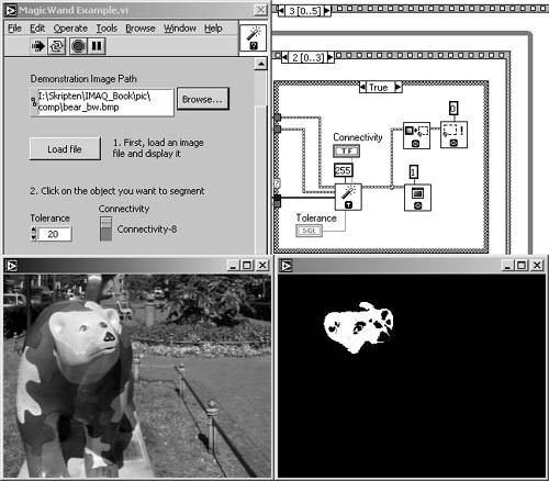
The next exercise is taken directly from IMAQ's own examples: IMAQ MagicWand . Just open the help window with the VI IMAQ MagicWand selected (you can find it in the Processing submenu) and click on MagicWand example; the example shown in Figure 4.78 is displayed.

Here, you can click on a region of a gray-scaled image, which most likely would be a particle after a thresholding operation. The result is displayed in a binary image and shows the selected object. Additionally, the object is highlighted in the original (gray-level) image by a yellow border. Figure 4.78 also shows the use of the IMAQ MagicWand function in the respective VI diagram.

Figure 4.78. IMAQ MagicWand: Separating Objects from the Background (National Instruments Example)

The last three functions in this section are similar to the analysis VIs we discuss in Chapter 5; they already supply some information about the particle structure of the image. Prepare the following exercise first.

Exercise 4.20: Skeleton Images.

Again, take one of the previous simple exercises, for example, Exercise 4.14, and replace its IMAQ Vision function by IMAQ Skeleton . You will need only a single control for the skeleton mode; with that control you select the Skeleton L, Skeleton M, or Skiz function. See Figure 4.79, showing a Skeleton L function, and Figure 4.80 for the results.

 

Figure 4.79. L-Skeleton Function

Figure 4.80. Diagram of Exercise 4.20

All skeleton functions work according to the same principle: they apply combinations of morphology operations (most of them are thinning functions) until the width of each particle is equal to 1 (called the skeleton line ). Other declarations for a skeleton function are these:

• The skeleton line shall be in (approximately) the center area of the original particle.
• The skeleton line shall represent the structure and the shape of the original particle. This means that the skeleton function of a coherent particle can only lead to a coherent skeleton line.

The L-skeleton function is based on the structuring element (see also [5]); the d in this mask means "don't care"; the element can be either 0 or 1 and produces the result shown in Figure 4.79.

Figure 4.81 shows the result of the M-skeleton function. Typically, the M-skeleton leads to skeleton lines with more branches, thus filling the area of the original particles with a higher amount. The M-skeleton function uses the structuring element [5].

Figure 4.81. M-Skeleton Function

The skiz function (Figure 4.82) is slightly different. Imagine an L-skeleton function applied not to the objects but to the background. You can try this with our Exercise 4.20. Modify it by adding an inverting function and compare the result of the Skiz function to the result of the L-skeleton function of the original image.

Figure 4.82. Skiz Function

Gray-Level Morphology

We return to the processing of gray-scaled images in the following exercises. Some morphology functions work not only with binary images, but also with images scaled according to the 8-bit gray-level set.

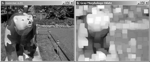
Exercise 4.21: Gray Morphology Functions.

Modify Exercise 4.13 by replacing the function IMAQ Morphology with IMAQ GrayMorphology . Add a digital control for Number of iterations and prepare your VI for the use of larger structuring elements, for example, 5 x 5 and 7 x 7.

You will need to specify the number of iterations for the erosion and dilation examples; larger structuring elements can be used in opening, closing, proper opening, and proper closing examples. See Figures 4.83 and 4.84 for results.

 

Gray-Level Erosion and Dilation

Figure 4.83 shows a gray-level erosion result after eight iterations (we need this large number of iterations here because significant results are not so easily visible in gray-level morphology). As an alternative, enlarge the size of your structuring element.

Figure 4.83. Gray Morphology: Erosion

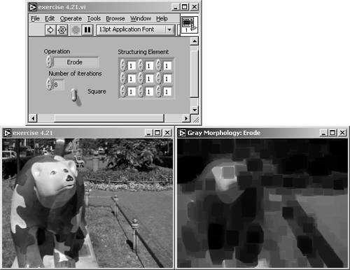
Figure 4.84. Diagram of Exercise 4.21

Of course, we have to modify the algorithm of the erosion function. In binary morphology, we set the center pixel value s to 0 if at least one of the other elements ( s i ) is equal to 0. Here we have gray-level values; therefore, we set s to the minimum value of all other coefficients s i :

Equation 4.44

 

The gray-level dilation is shown in Figure 4.85 and is now defined easily: s is set to the maximum value of all other coefficients s i :

Equation 4.45

 

Figure 4.85. Gray Morphology: Dilation

This exercise is a good opportunity to visualize the impact of different connectivity structures: square and hexagon. Figure 4.86 shows the same dilation result with square connectivity (left) and hexagon connectivity (right). The shape of the "objects" (it is not easy to talk of objects here because we do not have a binary image) after eight iterations is clearly determined by the connectivity structure.

Figure 4.86. Comparison of Square and Hexagon Connectivity

Gray-Level Opening and Closing

Also in the world of gray-level images, the opening function is defined as a (gray-level) erosion followed by a (gray-level) dilation using the same structuring element:

Equation 4.46

 

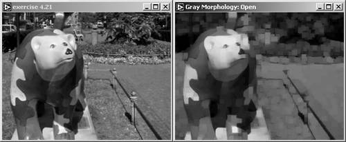
Figure 4.87 shows the result of a gray-level opening function.

Figure 4.87. Gray Morphology: Opening

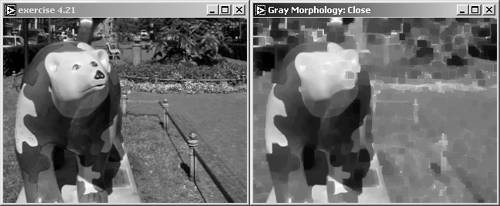
The result of a gray-level closing function can be seen in Figure 4.88. The gray-level closing function is defined as a gray-level dilation followed by a gray-level erosion using the same structuring element:

Figure 4.88. Gray Morphology: Closing

Equation 4.47

 

Gray-Level Proper Opening and Proper Closing

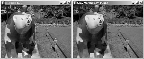
The two gray-level functions proper opening and proper closing are a little bit different from their binary versions. According to [4], gray-level proper opening is used to remove bright pixels in a dark surrounding and to smooth surfaces; the function is described by

Equation 4.48

 

note that the AND function of the binary version is replaced by a minimum function. A result is shown in Figure 4.89.

Figure 4.89. Gray Morphology: Proper Opening

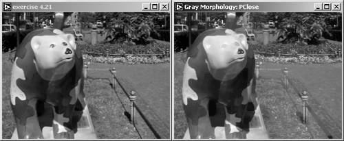
The gray-level proper closing function is defined as

Equation 4.49

 

a result is shown in Figure 4.90.

Figure 4.90. Gray Morphology: Proper Closing

Auto-Median Function

Compared to the binary version, the gray-level auto-median function also produces images with fewer details. The definition is different; the gray-level auto-median calculates the minimum value of two temporary images, both resulting from combinations of gray-level opening and closing functions:

Equation 4.50

 

See Figure 4.91 for a result of the gray-level auto-median function.

Figure 4.91. Gray Morphology: Auto-Median Function

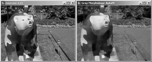
Image Analysis