Data Collection

Overview

Purpose of these tools

To help you collect reliable data that are relevant to the key questions you need to answer for your project

Deciding which tool to use

• Types of data, p. 70 to 71, discusses the types of data you may encounter, and how data type influences what analysis methods or tools you can and cannot use. Review as needed.
• Data collection planning, pp. 72 to 77, includes discussion of the measurement selection matrix (p. 74); stratification (p. 75); operational definitions (p. 76); and cautions on using existing data (p. 77). Use whenever you collect data.
• Checksheets, pp. 78 to 81, includes illustrations of different checksheets: basic (p. 79); frequency plot checksheet (p. 80); traveler (p 80); location (p 81). Review as needed.
• Sampling, pp. 81 to 86, discusses the basic (p. 81); factors in sample selection (p. 83), population and process sampling (p. 84), and determining minimum sample sizes (p. 85). Review recommended for all teams since almost all data collection involves sampling.
• Measurement System Analysis (including Gage R&R), pp. 87 to 99, covers the kind of data you need to collect (p. 89), and interpretation of the charts typically generated by MSA software programs (pp. 90 to 95); includes tips on checking bias (p. 95), stability (p. 97), and discriminatory power (p. 99). Recommended for all teams.
• Kappa calculations (MSA for attribute data), pp. 100 to 103, is recommended whenever you're collecting attribute data.

Types of data

1. Continuous

   Any variable measured on a continuum or scale that can be infinitely divided.

   There are more powerful statistical tools for interpreting continuous data, so it is generally preferred over discrete/attribute data.

   Ex: Lead time, cost or price, duration of call, and any physical dimensions or characteristics (height, weight, density, temperature)

2. Discrete (also called Attribute)

   All types of data other than continuous. Includes:

   • Count or percentage: Ex: counts of errors or % of output with errors.
   • Binomial data: Data that can have only one of two values. Ex: On-time delivery (yes/no); Acceptable product (pass/fail).
   • Attribute-Nominal: The "data" are names or labels. There is no intrinsic reason to arrange in any particular order or make a statement about any quantitative differences between them.

     Ex: In a company: Dept A, Dept B, Dept C

     Ex: In a shop: Machine 1, Machine 2, Machine 3

     Ex: Types of transport: boat, train, plane

   • Attribute-Ordinal: The names or labels represent some value inherent in the object or item (so there is an obvious order to the labels).

     Ex: On product performance: excellent, very good, good, fair, poor

     Ex: Salsa taste test: mild, hot, very hot, makes me suffer

     Ex: Customer survey: strongly agree, agree, disagree, strongly disagree

Note 

Though ordinal scales have a defined sequence, they do not imply anything about the degree of difference between the labels (that is, we can't assume that "excellent" is twice as good as "very good") or about which labels are good and which are bad (for some people a salsa that "makes me suffer" is a good thing, for others a bad thing)

Input vs output data

Output measures

Referred to as Y data. Output metrics quantify the overall performance of the process, including:

• How well customer needs and requirements were met (typically quality and speed requirements), and
• How well business needs and requirements were met (typically cost and speed requirements)

Output measures provide the best overall barometer of process performance.

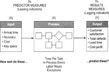
Process measures

One type of X variables in data. Measures quality, speed and cost performance at key points in the process. Some process measures will be subsets of output measures. For example, time per step (a process measure) adds up to total lead time (an output measure).

Input measures

The other type of X variables in data. Measures quality, speed and cost performance of information or items coming into the process. Usually, input measures will focus on effectiveness (does the input meet the needs of the process?).

Tips on using input and output data 

• The goal is to find Xs (Process and Input Measures) that are leading indicators of your critical output (Y)
  • That means the Xs will give you an early warning about potential problems with the Y
  • Such Xs are also key to finding root causes (the focus of the Analyze phase) and to catching problems before they become serious (Control phase)
• Use your SIPOC diagram and subprocess maps to help achieve a balance of both input and output measures
• Generally, you'll want to collect data on output measures at the start of your project to establish baselines
• Begin collecting data on at least one process and/or input measure early in the project to help generate initial data for Analyze

Data collection planning

Highlights

A good collection plan helps ensure data will be useful (measuring the right things) and statistically valid (measuring things right)

To create a data collection plan…

1. Decide what data to collect
   • If trying to assess process baseline, determine what metrics best represent overall performance of the product, service, or process
   • Find a balance of input (X) factors and output (Y) metrics (see p. 71)
   • Use a measurement selection matrix (p. 74) to help you make the decision
   • Try to identify continuous variables and avoid discrete (attribute) variables where possible since continuous data often convey more useful information

   Data Collection Plan

   Metric	Stratification factors	Operational definition	Sample size	Source and location	Collection method	Who will collect data
   How will data be used?				How will data be displayed?
   Examples: Identification of largest contributors Checking normality Identifying sigma level and variation Root cause analysis Correlation analysis				Examples: Pareto chart Histogram Control chart Scatter diagrams

2. Decide on stratification factors
   • See p. 75 for details on identifying stratification factors
3. Develop operational definitions
   • See p. 76 for details on creating operational definitions
4. Determine the needed sample size
   • See p. 81 for details on sampling
5. Identify source/location of data
   • Decide if you can use existing data or if you need new data (see p. 77 for details)
6. Develop data collection forms/checksheets
   • See pp. 78 to 81
7. Decide who will collect data

   Selection of the data collectors usually based on…

   • Familiarity with the process
   • Availability/impact on job
     • Rule of Thumb: Develop a data collection process that people can complete in 15 minutes or less a day. That increases the odds it will get done regularly and correctly.
   • Avoiding potential bias: Don't want a situation where data collectors will be reluctant to label something as a "defect" or unacceptable output
   • Appreciation of the benefits of data collection. Will the data help the collector?
8. Train data collectors
   • Ask data collectors for advice on the checksheet design.
   • Pilot the data collection procedures. Have collectors practice using the data collection form and applying operational definitions. Resolve any conflicts or differences in use.
   • Explain how data will be tabulated (this will help the collectors see the consequences of not following the standard procedures).
9. Do ground work for analysis
   • Decide who will compile the data and how
   • Prepare a spreadsheet to compile the data
   • Consider what you'll have to do with the data (sorting, graphing, calculations) and make sure the data will be in a form you can use for those purposes
10. Execute your data collection plan

Measurement selection matrix

Highlights

Used to find the measures most strongly linked to customer needs

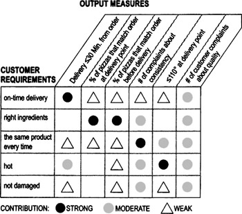
To create and use a measurement system matrix…

1. Collect VOC data (see Chapter 4) to identify critical-to-quality requirements. List down the side of a matrix.
2. Identify output measures (through brainstorming, data you're already collecting, process knowledge, SIPOC diagram, etc.) and list across the top of the matrix.
3. Work through the matrix and discuss as a team what relationshipa particular measure has to the corresponding requirement: strong, moderate, weak, or no relationship. Use numbers or symbols (as in the example shown here) to capture the team's consensus.
4. Review the final matrix. Develop plans for collecting data on the measures that are most strongly linked to the requirements.

Stratification factors

Highlights

Purpose is to collect descriptive information that will help you identify important patterns in the data (about root causes, patterns of use, etc.)

• Helps to focus the project on the critical few
• Speeds up the search for root causes
• Generates a deeper understanding of process factors

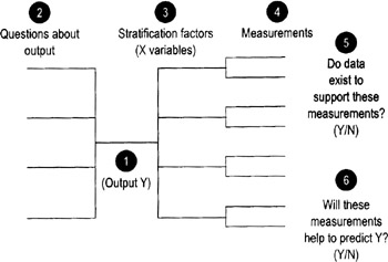
To identify stratification factors…

Your team can identify stratification by brainstorming a list of characteristics or factors you think may influence or be related to the problem or outcome you're studying. The method described here uses a modified tree diagram (shown above) to provide more structure to the process.

1. Identify an Output measure (Y), and enter it in the center point of the tree diagram.
2. List the key questions you have about that output.
3. Identify descriptive characteristics (the stratification factors) that define different subgroups of data you suspect may be relevant to your questions. These are the different ways you may want to "slice and dice" the data to uncover revealing patterns.

   Ex: You suspect purchasing patterns may relate to size of the purchasing company, so you'll want to collect information about purchaser's size

   Ex: You wonder if patterns of variation differ by time of day, so data will be labeled according to when it was collected

   Ex: You wonder if delays are bigger on some days of the week than on other days, so data will be labeled by day of week

4. Create specific measurements for each subgroup or stratification factor.
5. Review each of the measurements (include the Y measure) and determine whether or not current data exists.
6. Discuss with the team whether or not current measurements will help to predict the output Y. If not, think of where to apply measurement systems so that they will help you to predict Y.

Operational definitions

Highlights

• Operational definitions are clear and precise instructions on how to take a particular measurement
• They help ensure common, consistent data collection and interpretation of results

To create operational definitions…

1. As a team, discuss the data you want to collect. Strive for a common understanding of the goal for collecting that data.
2. Precisely describe the data collection procedure.
   • What steps should data collectors use?
   • How should they take the measurement?

     Ex: If measuring transaction time in a bank, what is the trigger to "start the stopwatch"? When a customer gets in line? When he or she steps up to a teller?

     Ex: If measuring the length of an item, how can you make sure that every data collector will put the ruler or caliper in the same position on the item?

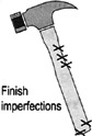
     Ex: What counts as a "scratch" on a product finish? What counts as an "error" on a form? (Misspellings? missing information? incorrect information?)

   • What forms or instruments will data collectors have to help them? Specifically how are these forms or instruments to be used?
   • How will the data be recorded? In what units?
3. Test the operational definition first with people involved in Step 2 above and then again with people not involved in the procedure, and compare results. Does everyone from both groups get the same result when counting or measuring the same things? Refine the measurement description as needed until you get consistent results.

Tip 

• Develop visual guides to help people take the measurements correctly—such as photos with notes on what is to be measured or counted (and how), "good" vs. "bad" standard examples, etc.

Cautions on using existing data

Using existing data lets you take advantage of archived data or current measures to learn about the output, process or input. Collecting new data means recording new observations (it may involve looking at an existing metric but with new operational definitions).

Using existing data is quicker and cheaper than gathering new data, but there are some strong cautions:

• The data must be in a form you can use
• Either the data must be relatively recent or you must be able to show that conditions have not changed significantly since they were collected
• You should know when and how the data were collected (and that it was done in a way consistent with the questions you want to answer)
• You should be confident that the data were collected using procedures consistent with your operational definition
• They must be truly representative of the process, group, measurement system
• There must be sufficient data to make your conclusions valid

If any of these conditions are not met, you should strongly think about collecting new data.

Tip 

• It's seldom wise to use old data only. Existing data is best used to establish historical patterns and to supplement new data.

Making a checksheet

Highlights

• Design a new checksheet every time you collect data (tailored to that situation)
• Having standard forms makes it easy to collect reliable, useful data
  • Enables faster capture and compiling of data
  • Ensures consistent data from different people
  • Captures essential descriptors (stratification factors) that otherwise might be overlooked or forgotten

To create and use a checksheet…

1. Select specific data and factors to be included
2. Determine time period to be covered by the form
   • Day, week, shift, quarter, etc.
3. Construct the form
   • Review different formats on the following pages and pick one that best fits your needs
   • Include a space for identifying the data collector by name or initials
   • Include reason/comment columns
   • Use full dates (month, date, year)
   • Use explanatory title
   • Decide how precise the measurement must be (seconds vs. minutes vs. hours; microns vs. millimeters) and indicate it on the form
     • Rule of thumb: smaller increments give better precision, but don't go beyond what is reasonable for the item being measured (Ex: don't measure in second a cycle time that last weeks—stick to hours)
4. Pilot test the form design and make changes as needed
   • If the "Other" column gets too many entries, you may be missing out on important categories of information. Examine entries classified as "Other" to see if there are new categories you could add to the checksheet.
   • Make changes before you begin the actual data collection trial

Basic checksheets

	Week
Defect	1	2	3	4	Total
Incorrect SSN	|		|	|	3
Incorrect Address		|			1
Incorrect Work History	|			|	2
Incorrect Salary History	∥	|	∥|	∥	8

• Easy to make and use
• Simply list the problems you're tracking and leave space to allow marks whenever someone finds that problem
• The example shown here also includes a time element

Frequency plot checksheet

• Easy to do by hand while a process is operating

  Repair shop output rate (Jul 1–Jul 19)
  Date	Completed repairs
  1
  2	X	X	X	X	X	X	X
  3	X	X	X	X	X
  4	X	X	X	X	X
  5	X	X	X	X
  6	X	X
  7	X	X	X
  8	X
  9	X	X	X	X	X	X
  10	X	X	X	X
  11	X	X	X	X
  12	X	X	X	X
  13	X
  14	X	X	X
  15
  16	X	X	X	X	X	X
  17	X	X	X	X	X
  18	X	X	X	X	X	X	X	X
  19	X	X	X	X

• Automatically shows distribution of items or events along a scale or ordered quantity
• Helps detect unusual patterns in a population or detect multiple populations
• Gives visual picture of average and range without any further analysis

Traveler checksheet

• A checksheet that travels with a work item (product, form, etc.). At each process step, the operator enters the appropriate data.
• Good way to collect data on process lead time.

  

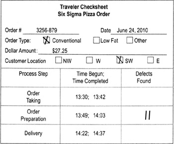
• Add columns as needed for other data, such as value-add time, delays, defects, work-in-process, etc.
• Put spaces for tracking information (a unique identifier for the job or part) at the top of the form
• Decide how the form will follow the work item (Ex: physically attached to paperwork or product, email alerts)

Location checksheet

• Data collection sheet based on a physical representation of a product, workplace, or form
• Data collectors enter marks where predefined defects occur
• Allows you to pinpoint areas prone to defects or problems (and therefore focuses further data collection efforts)

Sampling basics

Sampling is taking data on one or more subsets of a larger group in order to make decisions about the whole group.

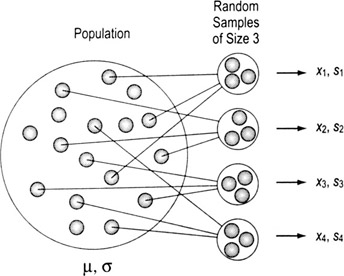
The trade-off is faster data collection (because you only have to sample) vs. some uncertainty about what is really going on with the whole group

The table to the right shows standard notations

	Population (= parameter)	Sampling (= statistic)
Count of items	N	n
Mean	μ	X
Mean estimator		X
Median
Std. Deviation	σ	s
Std. Dev. estimator		s
Note  Technically, the Xbar symbols should be written with lower-case letters, but (except for statistics books) are more often seen with capitals, so that is the convention used in this book
μ = the Greek letter "mu"	σ = the Greek letter "sigma"
—a straight line is called a "bar" and denotes an average	~ the curvy-line tilde (pronounced til-dah) denotes a median	ˆ a carat (or hat) denotes an estimator

Types of sampling process vs population

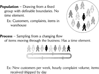
Why it matters whether you have process or population samples

• There are different tools for analyzing population data than for process data, so you must be clear about what kind of data you're gathering.
• Most traditional statistical training focuses on sampling from populations, where you have a nonchanging set of items or events from which it's relatively easy to select a representative sample. In contrast, quality and business process improvement tends to focus more often on processes, where change is a constant.
• Process data give more information (on trends, for example) than population data, so are preferred in most cases. Process sampling techniques are also the foundation of process monitoring and control.

Sampling terms

Sampling event—The act of extracting items from the population or process to measure.

Subgroup—The number of consecutive units extracted for measurement in each sampling event. (A "subgroup" can be just one item, but is usually two or more.)

Sampling Frequency—The number of times a day or week a sample is taken (Ex: twice per day, once per week). Applies only to process sampling.

Factors in sample selection

A number of factors affect the size and number of samples you must collect:

• Situation: Whether it is an existing set of items that will not change (a population) or a set that is continually changing (process)
• Data type: Continuous or discrete
• Objectives: What you'll do with results
• Familiarity: How much prior knowledge you have about the situation (such as historical data on process performance, knowledge of various customer segments, etc.)
• Certainty: How much "confidence" you need in your conclusions

Understanding bias

The big pitfall in sampling is bias—selecting a sample that does NOT really represent the whole. Typical sources of bias include:

• Self-selection (Ex: asking customers to call in to a phone number rather than randomly calling them)
• Self-exclusion (Ex: some types of customers will be less motivated to respond than others)
• Missing key representatives
• Ignoring nonconformances (things that don't match expectations)
• Grouping

Two worst ways to choose samples

• Judgment: choosing a sample based on someone's knowledge of the process, assuming that it will be "representative." Judgment guarantees a bias, and should be avoided.
• Convenience: sampling the items that are easiest to measure or at times that are most convenient. (Ex: collecting VOC data from people you know, or when you go for coffee).

Two best ways to choose samples

• Random: Best method for Population situations. Use a random number table or random function in Excel or other software, or draw numbers from a hat that will tell you which items from the population to select.
• Systematic: Most practical and unbiased in a Process situation. "Systematic" means that we select every nth unit. The risk of bias comes when the selection of the sample matches a pattern in the process.

Stable process (and population) sampling

Highlights

• A stable process is one that has only common cause variation (see Chapter 7). That means the same factors are always present and you don't need to worry about missing special causes that may come or go.
• In essence, a stable process is the same as a population.

To sample from a stable process…

1. Develop an initial profile of the data
   • Population size (N)
   • Stratification factors: If you elect to conduct a stratified sample, you need to know the size of each subset or stratum
   • Precision: how tightly (within what range of error) you want your measurement to describe the result
   • Estimate of the variation:
     • For continuous data, estimate the standard deviation of the variable being measured
     • For discrete data, estimate P, the proportion of the population that has the characteristic in question
2. Develop a sampling strategy
   • Random or systematic?
   • How will you draw the samples? Who will do it?
   • How will you guard against bias? (see p. 95)
     • You want the sample to be very representative but there is a cost in terms of time, effort, and dollars
     • The goal is to avoid differences between the items represented in the sample and those not in the sample
3. Determine the minimum sample size (see p. 85)
4. Adjust as needed to determine actual sample size

Tip 

• By definition an unstable process is unpredictable. Making inferences about a population based on a sample of an unstable process is ill-advised. Establish stability before making inferences.

Formulas for determining minimum sample size (population or stable process)

Continuous data

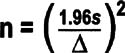
• n = minimum sample size
• 1.96 = constant representing a 95% confidence interval
• s = estimate of standard deviation data
• Δ= the difference (level of precision desired from the sample) you're trying to detect, in the same units as "s"

If you're using Minitab, it can calculate the sample size. Open Minitab, go to Stat > Power and Sample Size > then choose either…

1. 1-Sample t, if sample comes from a normally distributed data set and you want a relatively small sample (less than 25)
2. 1-Sample Z, if you are not sure about the distribution of your data set and a sample size greater than 30 is acceptable

You must tell Minitab what difference (Δ, delta) you are trying to detect and what power you are comfortable with (typically not less than 0.9) before a sample size can be calculated.

Discrete data sample size

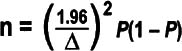
• n = minimum sample size
• P = estimate of the proportion of the population or process that is defective
• Δ = level of precision desired from the sample (express as a decimal or percentage, the same unit as P)
  • 1.96 = constant representing a 95% confidence interval
  • The highest value of P(1 − P) is 0.25, which is equal to P = 0.5

Again, Minitab can calculate the sample size. Open Minitab, go to Stat > Power and Sample Size > then choose either…

• 1 Proportion (comparing a proportion against a fixed standard)
• 2 Proportions (comparing 2 proportions)

For small populations

Changes in the minimum sample size are required for small populations. If n/N is greater than 0.05, the sample size can be adjusted to:

The proportion formula should be used only when: nP ≥5

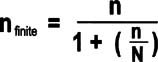
Both sample size formulas assume a 95% confidence interval and a small sample size (n) compared to the entire population size (N).

Measurement System Analysis (MSA) and Gage R R Overview

Purpose

To determine if a measurement system can generate accurate data, and if the accuracy is adequate to achieve your objectives

Why use MSA

• To make sure that the differences in the data are due to actual differences in what is being measured and not to variation in measurement methods

• Note 

  Experience shows that 30% to 50% of measurement systems are not capable of accurately or precisely measuring the desired metric

Types of MSA

• Gage R&R (next page)
• Bias Analysis (see p. 95)
• Stability Analysis (see p. 97)
• Discrimination Analysis (see p. 99)
• Kappa Analysis (see p.100)

Components of measurement error

Measurements need to be "precise" and "accurate." Accuracy and precision are different, independent properties:

• Data may be accurate (reflect the true values of the property) but not precise (measurement units do not have enough discriminatory power)
• Vice versa, data can be precise yet inaccurate (they are precisely measuring something that does not reflect the true values)
• Sometimes data can be neither accurate nor precise
• Obviously, the goal is to have data that are both precise and accurate

From a statistical viewpoint, there are four desirable characteristics that relate to precision and accuracy of continuous data:

1. No systematic differences between the measurement values we get and the "true value" (lack of bias, see p. 95)
2. The ability to get the same result if we take the same measurement repeatedly or if different people take the same measurement (Gage R&R, see p. 87)
3. The ability of the system to produce the same results in the future that it did in the past (stability, see p. 97)
4. The ability of the system to detect meaningful differences (good discrimination, see p. 99)

(Another desirable characteristic, linearity—the ability to get consistent results from measurement devices and procedures across a wide range of uses—is not as often an issue and is not covered in this book.)

Note 

Having uncalibrated measurement devices can affect all of these factors. Calibration is not covered in this book since it varies considerably depending on the device. Be sure to follow established procedures to calibrate any devices used in data collection.

Gage R R Collecting the data

Highlights

Gage R&R involves evaluating the reliability and repeatability of a measurement system.

• Repeatability refers to the inherent variability of the measurement system. It is the variation that occurs when successive measurements are made under the same conditions:
  • Same person
  • Same thing being measured
  • Same characteristic
  • Same instrument
  • Same set-up
  • Same environmental conditions
• Reproducibility is the variation in the average of the measurements made by different operators using the same measuring instrument and technique when measuring the identical characteristic on the same part or same process.
  • Different person
  • Same part
  • Same characteristic
  • Same instrument
  • Same setup
  • Same environmental conditions

To use Gage R R…

1. Identify the elements of your measurement system (equipment, operators or data collectors, parts/materials/process, and other factors).
   • Check that any measuring instruments have a discrimination that is equal to or less than 1/10 of the expected process variation/specification range
2. Select the items to include in the Gage R&R test. Be sure to represent the entire range of process variation. (Good and Bad over the entire specification plus slightly out of spec on both the high and low sides).
3. Select 2 or 3 operators to participate in the study.
4. Identify 5 to 10 items to be measured.
   • Make sure the items are marked for ease of data collection, but remain "blind" (unidentifiable) to the operators
5. Have each operator measure each item 2 to 3 times in random sequence.
6. Gather data and analyze. See pp. 90 to 95 for interpretation of typical plots generated by statistical software.

Tips 

• In manufacturing you may want to start with one of the Automotive Industry Action Group (see http://www.AIAG.org) standards…
  • short form: 2 operators measuring 5 items 2 times (= 20 measurements total)
  • long form: 3 operators measuring 10 items 3 times (= 90 measurements total)
• Be there for the study—NOT as a participant, but as an observer. Watch for unplanned influences.
• Randomize the items continuously during the study to prevent operator bias from influencing the test.
• When checking a given measurement system for the first time, let the process run as it normally would (no pre-training, no adjustment of equipment or instruments, no special items).

Interpreting Gage R R Results

Background

In most cases, the data you gather for an MSA or Gage R&R study will be entered in a software program. What follows are examples of the types of output you're likely to see, along with guidance on what to look for.

Basic terminology

Gage R&R = Gage system's Repeatability (the variation attributable to the equipment) and Reproducibility (the variation attributable to the personnel)

Measures the variability in the response minus the variation due to differences in parts. This takes into account variability due to the gage, the operators, and the operator by part interaction.

Repeat: "Within the gage"—amount of difference that a single data collector/inspector got when measuring the same thing over and over again.

Reprod: Amount of difference that occurred when different people measured the same item.

Part-to-Part: An estimate of the variation between the parts being measured.

Components of variation

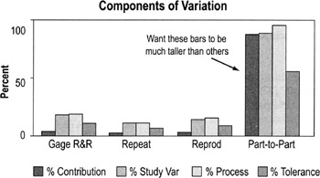
What you're looking for:

• You want the part-to-part bars to be much taller than the others because that means most of the variation is from true differences in the items being measured.
• If the Gage R&R, Repeat, and Reprod bars are tall, that means the measurement system is unreliable. (Repeat + Reprod = Gage R&R)
• Focus on the %Study Var bars—This is the amount of variation (expressed as a percentage) attributed to measurement error. Specifically, the calculation divides the standard deviation of the gage component by the total observed standard deviation then multiplies by 100. Common standards (such as AIAG) for %Study Var are:
  • Less than 10% is good—it means little variation is due to your measurement system; most of it is true variation
  • 10%-30% may be acceptable depending on the application (30% is maximum acceptable for any process improvement effort)
  • More than 30% unacceptable (your measurement system is too unpredictable)

Repeatability

Repeatability is checked by using a special time-series chart of ranges that shows the differences in the measurements made by each operator on each part.

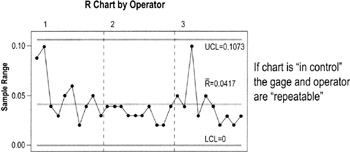
What you're looking for

• Is the range chart in control? (Review control chart guidelines, pp. 122 to 134)
• Any points that fall above the UCL need to be investigated
• If the difference between the largest value and the smallest value of the same part does not exceed the UCL, then that gage and operator may be considered Repeatable (depends on the application)

Reproducibility

Reproducibility is graphically represented by looking for significant differences between the patterns of data generated by each operator measuring the same items.

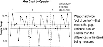
• Compare all the "Xbar chart by Operator" for all data collectors/operators used in the study
• Remember: the range chart determines the Xbar upper and lower control limits

What you're looking for:

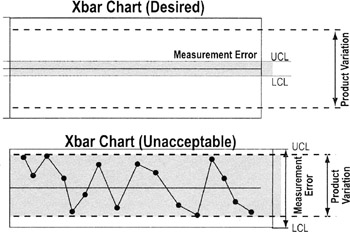
• This is one instance where you want the points to consistently go outside the upper and lower control limits (LCL, UCL). The control limits are determined by gage variance and these plots should show that gage variance is much smaller than variability within the parts.

  

• Also compare patterns between operators. If they are not similar, there may be significant operator/part or operator/equipment interactions (meaning different operators are using the equipment differently or measuring parts differently).

• Note 

  if the samples do not represent the total variability of the process, the gage (repeatability) variance may be larger than the part variance and invalidate the results here.

By Part chart

The By Part graph shows the data for the parts for all operators plotted together. It displays the raw data and highlights the average of those measurements. This chart shows the measurements (taken by three different operators) for each of 10 parts.

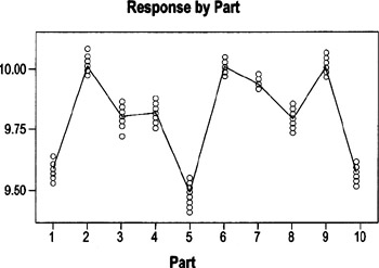
Want the range of readings for each part to be consistent with the range for other parts. That is NOT the case here (Ex: compare range for Part7 with range for Part3)

What you're looking for:

• The chart should show a consistent range of variation (smallest to the largest dimensions) for the same parts.
• If the spread between the biggest and smallest values varies a lot between different sets of points, that may mean that the parts chosen for the calibration were not truly representative of the variation within the process
• In this example, the spread between the highest and lowest value for Part 3 is much bigger than that for Part 7 (where points are closely clustered). Whether the difference is enough to be significant depends on the allowable amount of variation.

• Note 

  If a part shows a large spread, it may be a poor candidate for the test because the feature may not be clear or it may be difficult to measure that characteristic every time the same way.

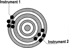
By Operator chart

The By Operator graph groups data by who was collecting the data ("running the process") rather than by part, so it will help you identify operator issues (such as inconsistent use of operational definitions or of measuring devices). In this example, each of three operators measured the same 10 parts. The 10 data points for each operator are stacked.

What you're looking for:

• The line connecting the averages (of all parts measured by an operator) should be flat or almost flat.

  

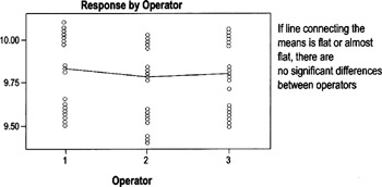
• Any significant slope indicates that at least one operator has a bias to measure larger or smaller than the other operators.
• In the example, Operator 2 tends to measure slightly smaller than Operators 1 and 3. Whether that is significant will depend on the allowable level of variation.

Operator*Part chart

This graph shows the data for each operator involved in the study. It is the best chart for exposing operator-and-part interaction (meaning differences in how different people measure different parts).

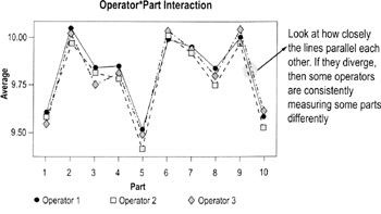
What you're looking for

• If the lines connecting the plotted averages diverge significantly, then there is a relationship between the operator making the measurements and the part being measured. This is not good and needs to be investigated.

MSA Evaluating bias

Accuracy vs bias

Accuracy is the extent to which the averages of the measurements deviate from the true value. In simple terms, it deals with the question, "On average, do I get the ‘right’ answer?" If the answer is yes, then the measurement system is accurate. If the answer is no, the measurement system is inaccurate.

Bias is the term given to the distance between the observed average measurement and the true value, or "right" answer.

In statistical terms, bias is identified when the averages of measurements differ by a fixed amount from the "true" value. Bias effects include:

Operator bias—Different operators get detectable different averages for the same value. Can be evaluated using the Gage R&R graphs covered on previous pages.

Instrument bias—Different instruments get detectably different averages for the same measurement on the same part. If instrument bias is suspected, set up a specific test where one operator uses multiple devices to measure the same parts under otherwise identical conditions. Create a "by instrument" chart similar to the "by part" and "by operator" charts discussed on pp. 94 to 95.

Other forms of bias—Day-to-day (environment), customer and supplier (sites). Talk to data experts (such as a Master Black Belt) to determine how to detect these forms of bias and counteract or eliminate them.

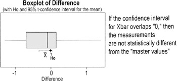
Testing overall measurement bias

1. Assemble a set of parts to be used for the test. Determine "master values" (the agreed-on measurement) for the characteristic for each part.
2. Calculate the difference between the measured values and the master value.
3. Test the hypothesis (see p. 156) that the average bias is equal to 0.
4. Interpret the position of 0 relative to the 95% confidence interval of the individual differences. You want the 95% confidence interval for the average to overlap the "true" value. In the boxplot below; the confidence interval overlaps the H0 value, so we cannot reject the null hypothesis that the sample is the same as the master value.

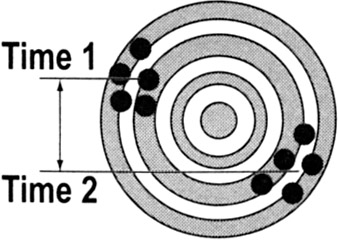
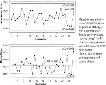
MSA Evaluating stability

If measurements do not change or drift over time, the instrument is considered to be stable. Loss of stability can be due to:

• deterioration of measurement devices
• increase in variability of operator actions (such as people forgetting to refer to operational definitions)

A common and recurring source of instability is the lack of enforced Standard Operating Procedures. Ask:

• Do standard operating procedures exist?
• Are they understood?
• Are they being followed?
• Are they current?
• Is operator certification performed?
• How and how often do you perform audits to test stability?

Measurement System stability can be tested by maintaining a control chart on the measurement system (see charts below).

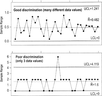
MSA Evaluating discrimination

Discrimination is the measurement system's ability to detect changes in the characteristic. A measurement system is unacceptable if it cannot detect the variation of the process, and/or cannot differentiate between special and common cause levels of variation. (Ex: A timing device with a discrimination of 1/100th of a second is needed to evaluate differences in most track events.)

In concept, the measurement system should be able to divide the smaller of the tolerance or six standard deviations into at least five data categories. A good way to evaluate discrimination graphically is to study a range chart. (The distance between the UCL and LCL is approximately 6 standard deviations.)

MSA for attribute discrete data

Attribute and ordinal measurements often rely on subjective classifications or ratings.

• Ex: Rating features as good or bad, rating wine bouquet, taste, and aftertaste; rating employee performance from 1 to 5; scoring gymnastics

The Measurement System Analysis procedures described previously in this book are useful only for continuous data. When there is no alternative—when you cannot change an attribute metric to a continuous data type—a calculation called Kappa is used. Kappa is suitable for non-quantitative (attribute) systems such as:

• Good or bad
• Go/No Go
• Differentiating noises (hiss, clank, thump)
• Pass/fail

Notes on Kappa for Attribute Data

1. Treats all non-acceptable categories equally

   Ex: It doesn't matter whether the numeric values from two different raters are close together (a 5 vs. a 4, for instance) or far apart (5 vs. 1). All differences are treated the same.

   Ex: A "clank" is neither worse nor better than a "thump"

2. Does not assume that the ratings are equally distributed across the possible range

   Ex: If you had a "done-ness" rating system with 6 categories (raw, rare, medium rare, medium, medium well, well done), it doesn't matter whether each category is "20% more done" than the prior category or if the done-ness varies between categories (which is a good thing because usually it's impossible to assign numbers in situations like this)

3. Requires that the units be independent
   • The measurement or classification of one unit is not influenced by any other unit
   • All judges or raters make classifications independently (so they don't bias one another)
4. Requires that the assessment categories be mutually exclusive (no overlap—something that falls into one category cannot also fall into a second category)

How to determine Kappa

1. Select sample items for the study.
   • If you have only two categories, good and bad, you should have a minimum of 20 good and 20 bad items (= 40 items total) and a maximum of 50 good and 50 bad (= 100 items total)
     • Try to keep approximately 50% good and 50% bad
     • Choose items of varying degrees of good and bad
   • If you have more than two categories, one of which is good and the other categories reflecting different defect modes, make 50% of the items good and have a minimum of 10% of the items in each defect mode.
     • You might combine some defect modes as "other"
     • The categories should be mutually exclusive (there is no overlap) or, if not, combine any categories that overlap
2. Have each rater evaluate the same unit at least twice.
3. Calculate a Kappa for each rater by creating separate Kappa tables, one per rater. (See instructions on next page.)
4. Calculate a between-rater Kappa by creating a Kappa table from the first judgment of each rater.
   • Between-rater Kappa will be made as Pairwise comparisons (A to B, B to C, A to C, etc.)
5. Interpret the results
   • If Kappa is lower than 0.7, the measurement system is not adequate
   • If Kappa is 0.9 or above, the measurement system is considered excellent
   • If P observed = P chance, then K=0
     • A Kappa of 0 indicates that the agreement is the same as that expected by random chance

   • Warning 

     One bad apple can spoil this bunch! A small Kappa means a rater must be changing how he/she takes the measurement each time (low repeatability). One rater with low repeatability skews the comparison with other raters.

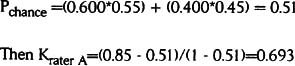
Doing the Kappa calculation

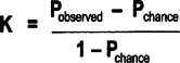
• Pobserved: Proportion of units on which both Raters agree = proportion both raters agree are good + the proportion both Raters agree are bad
• Pchance: Proportion of agreements expected by chance = (proportion that Rater A grades as good * proportion that Rater B grades as good) + (proportion that Rater A grades as bad * proportion that Rater B grades as bad)

Note 

This equation applies to a two-category (binary) analysis, where every item can fall into only one of two categories.

Example: Kappa for repeatability by a single Rater

		Rater A First Measure
		Good	Bad
		Rater A Second Measure	Good		0.5	0.1	0.6
Bad	0.05		0.35	0.4
		0.55	0.45

Pobserved is the sum of the probabilities on the diagonal:

Pchance is the probabilities for each classification multiplied and then summed:

This Kappa value is close to the generally accepted limit of 0.7.

Example: Kappa repeatability for comparing two different raters

Rater A to B comparison		Rater A First Measure
		Good	Bad
		Rater B First Measure	Good		9	3	12
Bad	2		6	8
		11	9

• 9 = Number of times both raters agreed the unit was good (using their first measurements)
• 3 = Number of times Rater A judged a unit bad and Rater B judged a unit good (using their first measurements)
• 2 = Number of times Rater A judged a unit good and Rater B judged a unit bad (using their first measurements)
• 6 = Number of times both raters agreed the unit was bad (using their first measurements)

This figures are converted to percentages:

Rater A to B comparison		Rater A First Measure
		Good	Bad
		Rater B First Measure	Good		0.45	0.15	0.6
Bad	0.1		0.3	0.4
		0.55	0.45

Pobserved is the sum of the probabilities on the diagonal:

Pchance is the probabilities for each classification multiplied and then summed:

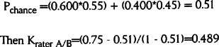
This Kappa value is well below the acceptable threshold of 0.7. It means that these two raters grade the items differently too often.