Creating Views in R/3
Creating Views in R 3
First we need to create two views: one for master data and one for texts.
Note
Views are ABAP dictionary objects. They are used to display data from multiple tables with specified table join conditions.
Work Instructions
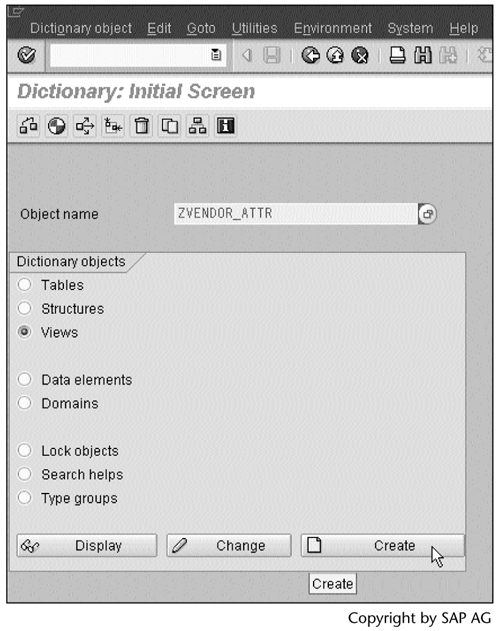
Step 1.To create a view for the master data, run transaction SE11, enter a name for the object, select the Views option in the Dictionary objects block, and then click  .
.
SCREEN 11.3
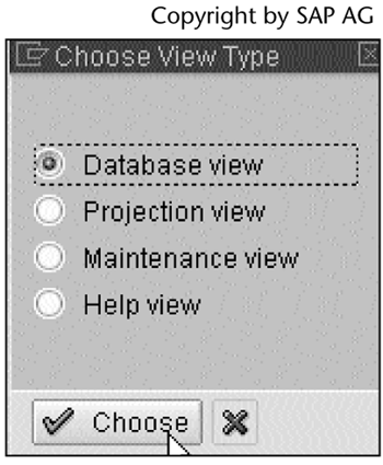
Step 2. Select the Database view option, and then click  .
.
SCREEN 11.4
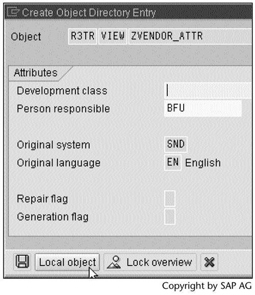
Step 3. The view needs to be included in a development class in order to be transported to other R/3 systems. In our example, we create views as local objects. Enter $TMP as the development class name and click the  , or simply click
  to assign the object to $TMP. Click
  to continue.
SCREEN 11.5
Note
A development class groups logically related objects, such as the objects that make up an accounting application. $TMP is a temporary local development class. Objects in $TMP cannot be transported into other systems.
See ABAP documents for more information on $TMP and non-$TMP development classes.
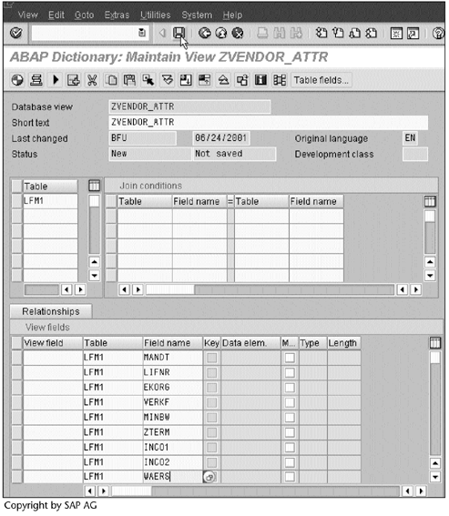
Step 4. This view consists of only one table, LFM1 (Vendor master record purchasing organization data). Enter the names of the fields from which we will extract data (see Table 11.1).
Click  to save the view definition.
SCREEN 11.6
Step 5. Click  to check the view definition. If it is valid, click
  to generate the view.
SCREEN 11.7
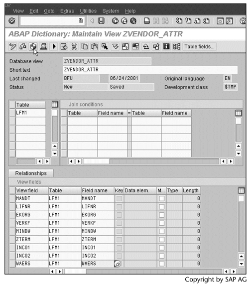
Step 6. To display the data selected by this view, select the Display data option on the Utilities menu.
SCREEN 11.8
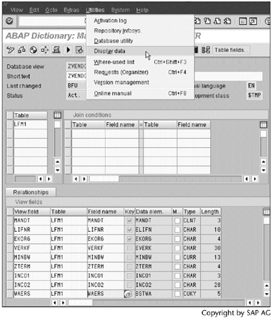
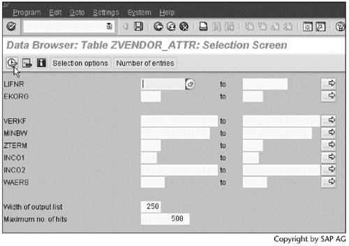
Step 7. Click  to display the data.
SCREEN 11.9
Result
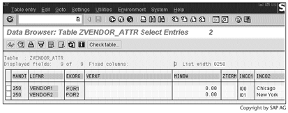
The result, which is shown in Screen 11.10, has two entries.
SCREEN 11.10
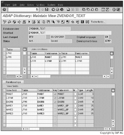
We use the same procedure to create a view for the text data (see Screen 11.11). This view consists of data from two tables, LFM1 (Vendor master record purchasing organization data) and LFA1 (Vendor master general section). The text data come from the LFA1 table.
SCREEN 11.11
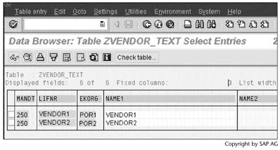
Screen 11.12 shows the data selected by this view, which consists of two entries as well.
SCREEN 11.12
Now we have created two views, one for master data and one for texts. Next, we will create DataSources using these two views.
Part I. Guided Tours
Business Scenario and SAP BW
- Business Scenario and SAP BW
- Sales Analysis A Business Scenario
- Basic Concept of Data Warehousing
- BW An SAP Data Warehousing Solution
- Summary
Creating an InfoCube
- Creating an InfoCube
- Creating an InfoArea
- Creating InfoObject Catalogs
- Creating InfoObjects Characteristics
- Creating InfoObjects Key Figures
- Creating an InfoCube
- Summary
Loading Data into the InfoCube
- Loading Data into the InfoCube
- Creating a Source System
- Creating an Application Component
- Creating an InfoSource for Characteristic Data
- Creating InfoPackages to Load Characteristic Data
- Checking Loaded Characteristic Data
- Entering the Master Data, Text, and Hierarchy Manually
- Creating an InfoSource for Transaction Data
- Creating Update Rules for the InfoCube
- Create an InfoPackage to Load Transaction Data
- Summary
Checking Data Quality
- Checking Data Quality
- Checking InfoCube Contents
- Using BW Monitor
- Using the Persistent Staging Area (PSA)
- Summary
Creating Queries and Workbooks
- Creating Queries and Workbooks
- Creating a Query Using BEx Analyzer
- Organizing Workbooks Using BEx Browser
- Using a Variable to Access a Hierarchy Node Directly
- Summary
Managing User Authorization
- Managing User Authorization
- Creating an Authorization Profile Using Profile Generator
- Creating an Authorization Object to Control User Access to the InfoCube Data
- Integrating Profile Generator and BEx Browser
- Summary
Part II. Advanced Topics
InfoCube Design
- InfoCube Design
- BW Star Schema
- InfoCube Design Alternative I Time-Dependent Navigational Attributes
- InfoCube Design Alternative II-Dimension Characteristics
- InfoCube Design Alternative III Time-Dependent Entire Hierarchies
- Other InfoCube Design Techniques
- Summary
Aggregates and Multi-Cubes
Operational Data Store (ODS)
- Operational Data Store (ODS)
- Creating an ODS Object
- Preparing to Load Data into the ODS Object, Then into an InfoCube
- Loading Data into the ODS Object
- Loading Data into the InfoCube
- Using 0RECORDMODE for Delta Load
- Summary
Business Content
- Business Content
- Creating an R/3 Source System
- Transferring R/3 Global Settings
- Replicating R/3 DataSources
- Installing Business Content Objects and Loading R/3 Data
- Summary
Generic R/3 Data Extraction
- Generic R/3 Data Extraction
- Creating Views in R/3
- Creating DataSources in R/3 and Replicating Them to BW
- Creating a Characteristic in BW
- Loading Data from R/3 into BW
- Summary
Data Maintenance
Performance Tuning
- Performance Tuning
- BW Statistics
- System Administration Assistant
- Tuning Query Performance
- Tuning Load Performance
- Summary
Object Transport
Appendix A. BW Implementation Methodology
Object Transport
Appendix B. SAP Basis Overview
Object Transport
- Object Transport
- Section B.1. SAP Basis 3-Tier Architecture
- Section B.2. Dispatcher, Work Processes, and Services
- Section B.3. Memory Management
Appendix C. Glossary
Appendix D. Bibliography
EAN: N/A
Pages: 106
