The PTR Submodel

Although the Rayleigh model, which covers all phases of the development process, can be used as the overall defect model, we need more specific models for better tracking of development quality. For example, the testing phases may span several months. For the waterfall process we used in previous examples, formal testing phases include component test, component regression test, and system test. For in-process quality management, one must also ensure that the chronological pattern of testing defect removal is on track. To derive a testing defect model, once again the Rayleigh model or other parametric models can be used if such models adequately describe the testing defect arrival patterns.

If the existing parametric models do not fit the defect patterns, special models for assessing in-process quality have to be developed. Furthermore, in many software projects, there is a common practice that the existing reliability models may not be able to address: the practice of continual code integration. As discussed in the previous section, sequential chunks of code are integrated when ready and this integration occurs throughout the development cycle until the system testing starts. To address this situation, we developed a simple nonparametric PTR submodel for testing defect tracking. It is called a PTR model because in many development organizations testing defects are tracked via some kind of problem tracking report (PTR), which is a part of the change control process during testing. Valid PTRs are, therefore, valid code defects. It is a submodel because it is part of the overall defect removal model. Simply put, the PTR submodel spreads over time the number of defects that are expected to be removed during the machine-testing phases so that more precise tracking is possible. It is a function of three variables :

1. Planned or actual lines of code integrated over time
2. Expected overall PTR rate (per thousand lines of code or per function point)
3. PTR- surfacing pattern after the code is integrated

The expected overall PTR rate can be estimated from historical data. Lines-of-code (LOC) integration over time is usually available in the current implementation plan. The PTR-surfacing pattern after code integration depends on both testing activities and the driver-build schedule. For instance, if a new driver is built every week, the PTR discovery/fix/integration cycle will be faster than that for drivers built biweekly or monthly. Assuming similar testing efforts, if the driver-build schedule differs from that of the previous release, adjustment to the previous release pattern is needed. If the current release is the first release, it is more difficult to establish a base pattern. Once a base pattern is established, subsequent refinements are relatively easy. For example, the following defect discovery pattern was observed for the first release of an operating system:

Month 1: 17%

Month 2: 22%

Month 3: 20%

Month 4: 16%

Month 5: 12%

Month 6: 9%

Month 7: 4%

To derive the PTR model curve, the following steps can be used:

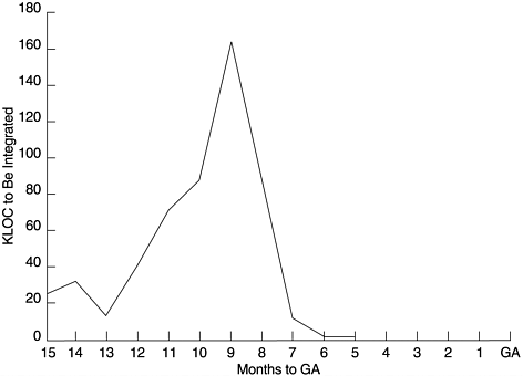
1. Determine the code integration plan; plot the lines of code (or amount of function points) to be integrated over time (see Figure 9.9).

   Figure 9.9. Planned KLOC Integration over Time of a Software Project

   

2. For each code integration, multiply the expected PTR rate by the KLOC for each planned integration to get the expected number of PTRs for each integration.
3. Spread over time the number of PTRs for each integration based on the PTR spread pattern and sum the number of PTRs for each time point to get the model curve.
4. Update the model when the integration plan (e.g., KLOC to be integrated over time) changes or actual integration data become available.
5. Plot the curve and track the current project in terms of months from the product's general availability (GA) date.

A calculator or a simple spreadsheet program is sufficient for the calculations involved in this model.

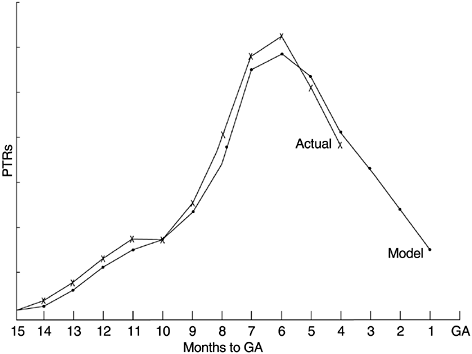
Figure 9.10 shows an example of the PTR submodel with actual data. The code integration changes over time during development, so the model is updated periodically. In addition to quality tracking, the model serves as a powerful quality impact statement for any slip in code integration or testing schedule. Specifically, any delay in development and testing will skew the model to the right, and the intersection of the model line and the imaginary vertical line of the product's ship date (GA date) will become higher.

Figure 9.10. PTR Submodel

Note that the PTR model is a nonparametric model and is not meant for projection. Its purpose is to enable the comparison of the actual testing defect arrival versus an expected curve for in-process quality management. Compared to the model curve, if the actual defect arrivals increase and peak earlier and decline faster relative to the product's ship date, that is positive, and vice versa. When data from the previous release of the same product are available, and the code integration over time is similar for the two releases, the simplest way to gauge the testing defect arrival pattern is to use the curve of the previous release as the model. One can also fit a software reliability model to the data to obtain a smooth model curve. Our experience indicates that the Rayleigh model, the Weibull distribution, the delayed S model and the inflection S model (see discussions in Chapter 8) are all candidate models for the PTR data. Whether the model fits the data, however, depends on the statistical goodness-of-fit test.

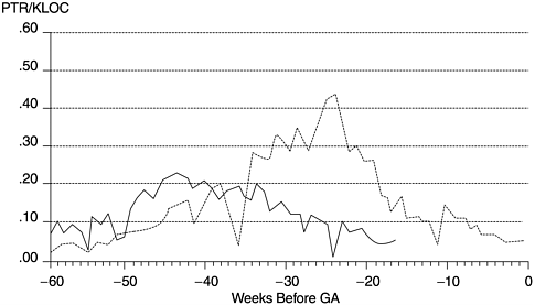
Figure 9.11 shows such a comparison. Given that the test coverage and effectiveness of the releases are comparable, the PTR arrival patterns suggest that the current release will have a substantially lower defect rate. The data points are plotted in terms of number of weeks before product shipment. The data points associated with an abrupt decline in the early and later segments of the curves represent Christmas week and July 4th week, respectively. In Chapter 10, we will discuss the PTR- related metrics with details in the context of software testing.

Figure 9.11. Testing Defect Arrival Patterns of Two Releases of a Product