Basic Assumptions

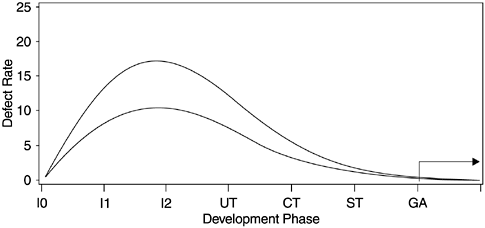
Using the Rayleigh curve to model software development quality involves two basic assumptions. The first assumption is that the defect rate observed during the development process is positively correlated with the defect rate in the field, as illustrated in Figure 7.3. In other words, the higher the curve (more area under it), the higher the field defect rate (the GA phase in the figure), and vice versa. This is related to the concept of error injection. Assuming the defect removal effectiveness remains relatively unchanged, the higher defect rates observed during the development process are indicative of higher error injection; therefore, it is likely that the field defect rate will also be higher.

Figure 7.3. Rayleigh Model Illustration I

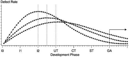
The second assumption is that given the same error injection rate, if more defects are discovered and removed earlier, fewer will remain in later stages. As a result, the field quality will be better. This relationship is illustrated in Figure 7.4, in which the areas under the curves are the same but the curves peak at varying points. Curves that peak earlier have smaller areas at the tail, the GA phase.

Figure 7.4. Rayleigh Model Illustration II

Both assumptions are closely related to the "Do it right the first time" principle. This principle means that if each step of the development process is executed properly with minimum errors, the end product's quality will be good. It also implies that if errors are injected, they should be removed as early as possible, preferably before the formal testing phases when the costs of finding and fixing the defects are much higher than that at the front end.

To formally examine the assumptions, we conducted a hypothesis-testing study based on component data for an AS/400 product. A component is a group of modules that perform specific functions such as spooling, printing, message handling, file handling, and so forth. The product we used had 65 components , so we had a good- sized sample. Defect data at high-level design inspection (I0), low-level design inspection (I1), code inspection (I2), component test (CT), system test (ST), and operation (customer usage) were available. For the first assumption, we expect significant positive correlations between the in-process defect rates and the field defect rate. Because software data sets are rarely normally distributed, robust statistics need to be used. In our case, because the component defect rates fluctuated widely, we decided to use Spearman's rank-order correlation. We could not use the Pearson correlation because correlation analysis based on interval data, and regression analysis for that matter, is very sensitive to extreme values, which may lead to misleading results.

Table 7.1 shows the Spearman rank-order correlation coefficients between the defect rates of the development phases and the field defect rate. Significant correlations are observed for I2, CT, ST, and all phases combined (I0, I1, I2, CT, and ST). For I0 and I1 the correlations are not significant. This finding is not surprising because (1) I0 and I1 are the earliest development phases and (2) in terms of the defect removal pattern, the Rayleigh curve peaks after I1.

Overall, the findings shown in Table 7.1 strongly substantiate the first assumption of the Rayleigh model. The significance of these findings should be emphasized because they are based on component-level data. For any type of analysis, the more granular the unit of analysis, the less chance it will obtain statistical significance. At the product or system level, our experience with the AS/400 strongly supports this assumption. As another case in point, the space shuttle software system developed by IBM Houston has achieved a minimal defect rate (the onboard software is even defect free). The defect rate observed during the IBM Houston development process (about 12 to 18 defects per KLOC), not coincidentally, is much lower than the industry average (about 40 to 60 defects per KLOC).

To test the hypothesis with regard to the second assumption of the Rayleigh model, we have to control for the effects of variations in error injection. Because error injection varies among components, cross-sectional data are not suitable for the task. Longitudinal data are better, but what is needed is a good controlled experi-ment. Our experience indicates that even developing different functions by the same team in different releases may be prone to different degrees of error. This is especially the case if one release is for a major-function development and the other release is for small enhancements.

Table 7.1. Spearman Rank Order Correlations

Phase	Rank-Order Correlation	n	Significance Level
I0	.11	65	Not significant
I1	.01	65	Not significant
I2	.28	65	.02
CT	.48	65	.0001
ST	.49	65	.0001
All (I0, I1, I2, CT, ST)	.31	65	.01

In a controlled experiment situation, a pool of developers with similar skills and experiences must be selected and then randomly assigned to two groups, the experiment group and the control group. Separately the two groups develop the same functions at time 1 using the same development process and method. At time 2, the two groups develop another set of functions, again separately and again with the same functions for both groups. At time 2, however, the experiment group intentionally does much more front-end defect removal and the control group uses the same method as at time 1. Moreover, the functions at time 1 and time 2 are similar in terms of complexity and difficulty. If the testing defect rate and field defect rate of the project by the experiment group at time 2 are clearly lower than that at time 1 after taking into account the effect of time (which is reflected by the defect rates of the control groups at the two times), then the second assumption of the Rayleigh model is substantiated.

Without data from a controlled experiment, we can look at the second assumption from a somewhat relaxed standard. In this regard, IBM Houston's data again lend strong support for this assumption. As discussed in Chapter 6, for software releases by IBM Houston for the space shuttle software system from November 1982 to December 1986, the early detection percentages increased from about 50% to more than 85%. Correspondingly, the product defect rates decreased monotonically by about 70% (see Figures 6.1 and 6.2 in Chapter 6). Although the error injection rates also decreased moderately, the effect of early defect removal is evident.