The Exponential Model
The exponential model is another special case of the Weibull family, with the shape parameter m equal to 1. It is best used for statistical processes that decline monotonically to an asymptote. Its cumulative distribution function (CDF) and probability density function (PDF) are
![]()
where c is the scale parameter, t is time, and l =1/ c . Applied to software reliability, l is referred to as the error detection rate or instantaneous failure rate . In statistical terms it is also called the hazard rate .
Again the preceding formulas represent a standard distribution ”the total area under the PDF curve is 1. In actual application, the total number of defects or the total cumulative defect rate K needs to be multiplied to the formulas. K and lambda ( l ) are the two parameters for estimation when deriving a specific model from a data set.
The exponential distribution is the simplest and most important distribution in reliability and survival studies. The failure data of much equipment and many processes are well described by the exponential distribution: bank statement and ledger errors, payroll check errors, light bulb failure, automatic calculating machine failure, radar set component failure, and so forth. The exponential distribution plays a role in reliability studies analogous to that of normal distribution in other areas of statistics.
In software reliability the exponential distribution is one of the better known models and is often the basis of many other software reliability growth models. For instance, Misra (1983) used the exponential model to estimate the defect-arrival rates for the shuttle's ground system software of the National Aeronautics and Space Administration (NASA). The software provided the flight controllers at the Johnson Space Center with processing support to exercise command and control over flight operations. Data from an actual 200- hour flight mission indicate that the model worked very well. Furthermore, the mean value function (CDF) of the Goel-Okumoto (1979) nonhomogeneous Poisson process model (NPPM) is in fact the exponential model.
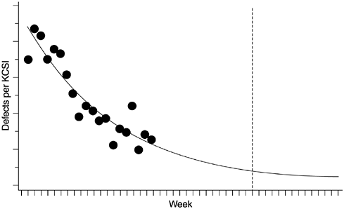
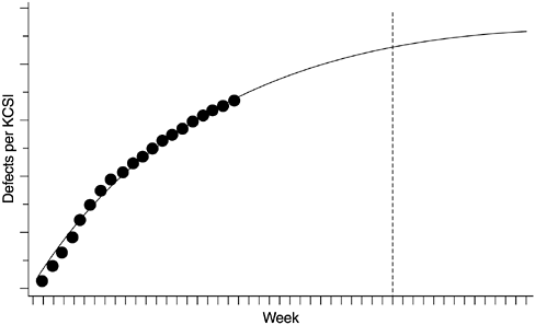
Figures 8.1 and 8.2 show the exponential model applied to the data of one of the AS/400 software products. We have modeled the weekly defect arrival data since the start of system test, when the development work was virtually complete. The system-testing stage uses customer interfaces, tests external requirements, and simulates end- user application environments. The pattern of defect arrivals during this stage, therefore, should be indicative of the latent defect rate when the system is shipped.
Figure 8.1. Exponential Model ”Density Distribution

Figure 8.2. Exponential Model ”Cumulative Distribution

Like the Rayleigh model, the exponential model is simple and quick to implement when powerful statistical software is available. For example, it can be implemented via SAS programs similar to the one shown in Figure 7.5 of the previous chapter. Of course, if a high degree of usability and various scenarios are desired, more elaborate software is needed.
Besides programming, the following should be taken into consideration when applying the exponential distribution for reliability projection or estimating the number of software defects. First, as with all types of modeling and estimation, the more accurate and precise the input data, the better the outcome. Data tracking for software reliability estimation is done either in terms of precise CPU execution time or on a calendar-time basis. Normally execution-time tracking is for small projects or special reliability studies; calendar-time tracking is common for commercial development. When calendar-time data are used, a basic assumption for the exponential model is that the testing effort is homogeneous throughout the testing phase. Ohba (1984) notes that the model does not work well for calendar-time data with a nonhomogeneous time distribution of testing effort. Therefore, this assumption must be examined when using the model. For instance, in the example shown in Figures 8.1 and 8.2 the testing effort remained consistently high and homogeneous throughout the system test phase; a separate team of testers worked intensively based on a predetermined test plan. The product was also large (>100 KLOC) and therefore the trend of the defect arrival rates tended to be stable even though no execution-time data were available.
To verify the assumption, indicators of the testing effort, such as the person-hours in testing for each time unit (e.g., day or week), test cases run, or the number of variations executed, are needed. If the testing effort is clearly not homogeneous, some sort of normalization has to be made. Otherwise, models other than the exponential distribution should be considered .
As an example of normalization, let us assume the unit of calendar time is a week and it is clear that the weekly testing effort is not homogeneous. Further assume that weekly data on the number of person-hours in testing are known. Simple adjustments such as the following can reduce artificial fluctuations in the data and can make the model work better:
- Accumulate the total person-hours in testing for the entire testing phase and calculate the average number of person-hours in testing per week, n.
- Starting from the beginning of testing, calculate the defect rates (or defect count) for each n person-hour units. Allocate the defect rates to the calendar week in sequence. Specifically, allocate the defect rate observed for the first n person-hours of testing to the first week; allocate the defect rate observed for the second n person-hours of testing to the second week, and so forth.
- Use the allocated data as weekly input data for the model.
Second, the more data points available, the better the model will perform ” assuming there is an adequate fit between the model and the data. The question is: When the test is in progress, how much data is needed for the model to yield reasonably adequate output? Ehrlich and associates (1990) investigated this question using data from AT&T software that was a transmission measurement system for remote testing of special service circuits. They assessed the predictive validity of the exponential model with data at 25%, 50%, 60%, 70%, and 80% into test, and at test completion. They found that at 25% into test the model results were way off. At 50% the results improved considerably but were still not satisfactory. At 60% into test, the exponential model had satisfactory predictive validity. Although it is not clear whether these findings can be generalized, they provide a good reference point for real-time modeling.
What Is Software Quality?
Software Development Process Models
- Software Development Process Models
- The Waterfall Development Model
- The Prototyping Approach
- The Spiral Model
- The Iterative Development Process Model
- The Object-Oriented Development Process
- The Cleanroom Methodology
- The Defect Prevention Process
- Process Maturity Framework and Quality Standards
Fundamentals of Measurement Theory
- Fundamentals of Measurement Theory
- Definition, Operational Definition, and Measurement
- Level of Measurement
- Some Basic Measures
- Reliability and Validity
- Measurement Errors
- Be Careful with Correlation
- Criteria for Causality
Software Quality Metrics Overview
- Software Quality Metrics Overview
- Product Quality Metrics
- In-Process Quality Metrics
- Metrics for Software Maintenance
- Examples of Metrics Programs
- Collecting Software Engineering Data
Applying the Seven Basic Quality Tools in Software Development
- Applying the Seven Basic Quality Tools in Software Development
- Ishikawas Seven Basic Tools
- Checklist
- Pareto Diagram
- Histogram
- Run Charts
- Scatter Diagram
- Control Chart
- Cause-and-Effect Diagram
- Relations Diagram
Defect Removal Effectiveness
- Defect Removal Effectiveness
- Literature Review
- A Closer Look at Defect Removal Effectiveness
- Defect Removal Effectiveness and Quality Planning
- Cost Effectiveness of Phase Defect Removal
- Defect Removal Effectiveness and Process Maturity Level
The Rayleigh Model
- The Rayleigh Model
- Reliability Models
- The Rayleigh Model
- Basic Assumptions
- Implementation
- Reliability and Predictive Validity
Exponential Distribution and Reliability Growth Models
- Exponential Distribution and Reliability Growth Models
- The Exponential Model
- Reliability Growth Models
- Model Assumptions
- Criteria for Model Evaluation
- Modeling Process
- Test Compression Factor
- Estimating the Distribution of Total Defects over Time
Quality Management Models
- Quality Management Models
- The Rayleigh Model Framework
- Code Integration Pattern
- The PTR Submodel
- The PTR Arrival and Backlog Projection Model
- Reliability Growth Models
- Criteria for Model Evaluation
- In-Process Metrics and Reports
- Orthogonal Defect Classification
In-Process Metrics for Software Testing
- In-Process Metrics for Software Testing
- In-Process Metrics for Software Testing
- In-Process Metrics and Quality Management
- Possible Metrics for Acceptance Testing to Evaluate Vendor-Developed Software
- How Do You Know Your Product Is Good Enough to Ship?
Complexity Metrics and Models
- Complexity Metrics and Models
- Lines of Code
- Halsteads Software Science
- Cyclomatic Complexity
- Syntactic Constructs
- Structure Metrics
- An Example of Module Design Metrics in Practice
Metrics and Lessons Learned for Object-Oriented Projects
- Metrics and Lessons Learned for Object-Oriented Projects
- Object-Oriented Concepts and Constructs
- Design and Complexity Metrics
- Productivity Metrics
- Quality and Quality Management Metrics
- Lessons Learned from OO Projects
Availability Metrics
- Availability Metrics
- 1 Definition and Measurements of System Availability
- Reliability, Availability, and Defect Rate
- Collecting Customer Outage Data for Quality Improvement
Measuring and Analyzing Customer Satisfaction
- Measuring and Analyzing Customer Satisfaction
- Customer Satisfaction Surveys
- Analyzing Satisfaction Data
- Satisfaction with Company
- How Good Is Good Enough
Conducting In-Process Quality Assessments
- Conducting In-Process Quality Assessments
- The Preparation Phase
- The Evaluation Phase
- The Summarization Phase
- Recommendations and Risk Mitigation
Conducting Software Project Assessments
- Conducting Software Project Assessments
- Audit and Assessment
- Software Process Maturity Assessment and Software Project Assessment
- Software Process Assessment Cycle
- A Proposed Software Project Assessment Method
Dos and Donts of Software Process Improvement
- Dos and Donts of Software Process Improvement
- Measuring Process Maturity
- Measuring Process Capability
- Staged versus Continuous Debating Religion
- Measuring Levels Is Not Enough
- Establishing the Alignment Principle
- Take Time Getting Faster
- Keep It Simple or Face Decomplexification
- Measuring the Value of Process Improvement
- Measuring Process Adoption
- Measuring Process Compliance
- Celebrate the Journey, Not Just the Destination
Using Function Point Metrics to Measure Software Process Improvements
- Using Function Point Metrics to Measure Software Process Improvements
- Software Process Improvement Sequences
- Process Improvement Economics
- Measuring Process Improvements at Activity Levels
Concluding Remarks
- Concluding Remarks
- Data Quality Control
- Getting Started with a Software Metrics Program
- Software Quality Engineering Modeling
- Statistical Process Control in Software Development
A Project Assessment Questionnaire
EAN: 2147483647
Pages: 176
