Quantifying and Analyzing Project Risk
Overview
"Knowledge is power."
—FRANCIS BACON
Information is central to managing projects successfully. Knowledge of the work and of the potential risk serves as the first and best defense against problems and project delay. The overall assessment of project risk provides concrete justification for necessary changes in the project objective, so it is one of the most powerful tools you have for failure-proofing difficult projects. Project-level risk rises steeply for projects with insufficient resources or excessively aggressive schedules, and risk assessments offer compelling evidence of the exposure this represents. Knowledge of project risk also sets expectations for the project appropriately, both for the deliverables and for the work that lies ahead.
Most of the content of this chapter falls into the "Qualitative Risk Analysis" and "Quantitative Risk Analysis" portions of the Planning Processes in the PMBOK Guide. The focus of this chapter is the analysis of overall project risk, building on the foundation of analysis and response planning for known activity risks discussed in the two preceding chapters. The principal ideas covered in this chapter include:
- Project-level risk
- Aggregated risk responses
- Questionnaires and surveys
- Project simulation and modeling
- Analysis of scale
- Project appraisals
- Project metrics
- Financial metrics
Project Level Risk
Considered one by one, the known risks on a project may seem relatively easy to deal with, or overwhelming, or somewhere in between. Managing risk at the activity level is necessary, but it is not sufficient; you also need to develop a sense of overall project risk. Overall project risk arises, in part, from all the activity-level data combined, but it also has a component that is more pervasive, coming from the project as a whole. High-level project risk assessment was discussed in Chapter 3, using methods that required only information available during initial project definition. Those high-level techniques—the risk framework, the risk complexity index, and the risk assessment grid—may also be reviewed and revised according to your project plans.
As the preliminary project planning process approaches completion, you have much more information available, so you can assess project risk more precisely and thoroughly. There are a number of useful tools for assessing project risk, including statistics, metrics, and modeling tools such as the Program Evaluation and Review Technique (PERT). Risk assessment using planning data may be used to support decisions and make recommendations for project changes, project control, and project execution.
Common Project Risks
Generic sources of project risk are many. In Assessment and Control of Software Risks, Capers Jones lists as the top five:
- Inadequate measures. If cost and effort measures are inaccurate or missing, there is little precision in project planning and high, uncontrolled costs.
- Excessive schedule pressure. Setting project deadlines too aggressively leads to poor quality, low morale, high attrition, and project cancellation.
- Management malpractice. Project leaders good at technical work but not skilled in definition, planning, estimating, tracking, communication, and project control produce poor results and very high levels of inefficiency.
- Creeping user requirements. Inadequate specification change control wastes money and effort and causes rework.
- Very large projects. Sheer size is a project risk; the larger the project, the more likely it is to end in cancellation. Jones reports that the largest projects are generally canceled a year or more after the original deadline, having spent at least double the intended budget, in most cases without providing any salvageable output.
Uses of Project Risk Data
As discussed in Chapter 1, risk information has many uses, including helping sponsors to select and compare potential projects. Project risk data can build support for less risky projects, and it may lead to cancellation of higher-risk projects. It can also be used in setting relative project priorities. High-risk projects may warrant lower priority. Raising project priority may significantly reduce project risk by opening doors, reducing obstacles, making resources available, and reducing queues. Risk assessment is also important in managing a portfolio of projects. The mix of ongoing projects should represent an appropriate risk profile, including both lower- and higher-risk projects in proportions consistent with business strategies. Without adequate project risk information, all these decisions will be made using guesswork.
Project risk assessment may also be used to reduce the risk of individual projects. Project-level risk assessments may reveal sources of project risk that are part of the project infrastructure. Fine-tuning the overall project by making structural and other changes can drop risk significantly. The overall assessment of risk also provides a data-driven justification for establishing management reserve for the project. Taking into account overall risk, managers may set the project objectives with aggressive targets, along with commitments and expectations that are less aggressive. The window between the aggressive target and the project's commitment can be sized to reflect project risk and uncertainty. For example, a target project schedule might call for completion of the project in twelve months, but taking risk analysis into consideration, it would not be late unless it requires more than fourteen months. Both schedule and resource reserves are common for risky projects.
Finally, project risk data are useful in communication. Documentation of project risk can be vital in discussions with sponsors and managers—it is harder for them to argue with facts and data than it is to argue with you. Risk information also builds awareness of project uncertainties on the project team.
The techniques, tools, ideas and metrics described in this chapter will assist you in all of this.
Aggregating Risk Responses
One way to measure project risk is to add up all the expected consequences for all of the contingency plans established for the project. This is not just a simple sum; the total is based on the estimated cost (or time) involved multiplied by the risk probability—the "loss times likelihood" for the whole project.
One way to calculate project-level risk is by accumulating the consequences of the contingency plans. To do this, you sum the expected costs for all the plans—their estimated costs weighted by the risk probabilities. Similarly, you can calculate the total expected project duration increase required by the contingency plans using the same probability estimates. For example, if a contingency plan associated with a risk having a 10 percent probability will cost $10,000 and slip the project by ten days, the contribution to the project totals will be $1,000 and one day, respectively.
Another way to generate similar data is by using the differences between PERT-based "expected" estimates and the "most likely" activity estimates. Summing these estimates of both cost and time impact for the project generates an assessment roughly equivalent to the contingency plan data.
While these sums of expected consequences provide a baseline for overall project risk, they tend to underestimate total risk, for a number of reasons. First, this analysis assumes that all project risks are independent, with no expected correlation. On real projects, this assumption is generally incorrect; some project risks are much more likely after other risks have occurred. Project activities are linked through common methodologies, staffing, and other factors. Second, a project has a limited staff, so whenever there is a problem, nearly all of the project leader's attention (and much of the project team's) will be on recovery. While distracted by problem solving, the project leader will focus much less on all the other project activities, making additional trouble elsewhere that much more likely.
Another big reason that overall project risk is underestimated using this method is that the sums do not yet account for project-level risk factors. Overall project-level risk factors include:
- Experience of project manager
- Weak sponsorship
- Reorganization, business changes
- Regulatory issues
- Lack of common practices (e.g., life cycle, planning)
- Market window or other timing assumptions
- Insufficient risk management
- Ineffective project decomposition, resulting in inefficient work flow
- Unfamiliar levels of project effort
- Low project priority
- Poor motivation and team morale
- Weak change management control
- Lack of customer interaction
- Communications issues
- Poorly defined infrastructure
- Inaccurate (or no) metrics
The first two factors on the list are particularly significant. If the project leader has little experience running similar projects successfully, or the project has low priority, or both, you can increment the overall project risk assessment from summing expected impacts by at least 10 percent for each. Similarly, make adjustments for any of the other factors that may be significant for the project. Even after these adjustments, the risk assessment will still be somewhat conservative, because the effect of any "unknown" risk in your project has not been included.
Compare the total expected project duration and cost impacts related to project risks with your preliminary baseline plan. Whenever the expected risk impact for either time or cost exceeds 20 percent of your plan, the project is very risky. You can use these data on cost and schedule risk to adjust your project plan, justify management reserve, or both.
Questionnaires and Surveys
Questionnaires and surveys are a well-established technique for assessing project risk. These can range from simple, multiple-response survey forms to assessments using computer spreadsheets or any other suitable format or computer tool. However a risk assessment tool is implemented, it will be most useful if you customize it for your project.
Many organizations have and use risk surveys. If there is a survey or questionnaire commonly used for projects similar to yours, it may require very little customizing, but it is always a good idea to review the questions and fine-tune the instrument before using it. If you do not have a standard survey format, the following example is a generic three-option risk survey that can be adapted for use on a wide range of technical projects.
This survey approach to risk assessment also works best when the number of total questions is kept to a minimum, so review the format you intend to use and select only the questions that are most relevant to your project risks. You may need to modify existing questions or to create new risk evaluation questions to maximize the usefulness of the survey for your project. It also helps to keep the responses simple. If you develop your own survey, limit the number of responses for each question to no more than four clearly worded responses.
Once you have finalized the risk assessment questionnaire, the next step is to get input from each member of the core project team. Ask each person who participated in project planning to respond to each question, and then collect their data.
Risk survey data are useful in two ways. First, you can analyze all the data to produce an overall assessment of risk. This can be used to compare projects, to set expectations, and to establish risk reserves. Second, you can scan the responses question by question to find particular risks—questions where the responses are consistently in the high-risk category. Risk surveys can be very compelling evidence for needed changes in project infrastructure or other project factors that increase risk. For high-risk factors, ask, "Do we need to settle for this? Is there any reason we should not consider changes that will reduce project risk?" Also, investigate any questions with widely divergent responses, and conduct additional discussions to establish common understanding within the project team.
Instructions for the Project Risk Questionnaire
The following document is a generic risk questionnaire, typical of surveys commonly used on technical projects. The results of using this sort of tool are qualitative and not intended to provide high-precision analysis of comparative risk between different projects.
Before using the following survey, read each one of the questions and make changes as needed to reflect your project environment. Strike out any questions that are irrelevant, and add new questions if necessary to reflect risky aspects of your project. Effective surveys are short, so delete any questions that seem less applicable. Section 2, "Technical Risks," normally requires the most intensive editing. The three sections focus on:
- Project external factors (such as users, budgets, and schedule constraints)
- Development issues (such as tools, software, and hardware)
- Project internal factors (such as infrastructure, team cohesion, and communications)
Add or delete questions in these categories to make this tool more useful to you.
To use the survey, distribute copies to key project contributors and stakeholders (at least one other person in addition to yourself), and ask each person to select one of the three choices offered for each question.
To interpret the information, assign values of 1 to selections in the first column, 3 to selections in the middle column, and 9 to selections in the third column. Within each section, sum up the responses, then divide each sum by the number of responses tallied. For example, if three people answered all seventeen questions in Section 1—for a total of fifty-one questions—and the weighted responses sum to 195, the result is 3.82, or medium risk. Within each section, use the following evaluation criteria:
|
Low risk: |
1.00–2.50 |
|
Medium risk: |
2.51–6.00 |
|
High risk: |
6.01–9.00 |
Average the three section results to determine overall project risk, using the same criteria. Although the results of this kind of survey are qualitative, they can help you to identify sources of high risk in your project. For any section with medium or high risk, consider changes to the project that might lower the risk. Within each section, look for responses in the third column. Brainstorm ideas, tactics, or project changes that could shift the response, reducing overall project risk.
Risk Questionnaire
For each question below, choose the response that best describes your project. If the best response seems to lie between two choices, check the one of the pair further to the right.
Section 1. Project Parameter and Target User Risks
|
|
|
|
|
|
|
|
|
|
|
|
|
|
|
|
|
|
|
|
|
|
|
|
|
|
|
|
|
|
|
|
|
|
|
|
|
|
|
|
|
|
|
|
|
|
|
|
|
|
|
Section 2. Technical Risks
General
|
|
|
|
|
|
|
|
|
|
|
|
|
|
|
|
|
|
|
|
|
Hardware
|
|
|
|
|
|
|
|
|
|
|
|
|
|
|
|
|
|
Software
|
|
|
|
|
|
|
|
|
|
|
|
|
|
|
|
|
|
Section 3. Structure Risks
|
|
|
|
|
|
|
|
|
|
|
|
|
|
|
|
|
|
|
|
|
|
|
|
|
|
|
|
|
|
|
|
|
|
|
|
|
|
|
|
|
|
|
|
|
|
|
|
|
|
|
|
|
|
|
|
|
|
|
|
|
|
|
|
|
|
|
|
|
Project Simulation and Modeling
The best-known project modeling methodology is the Program Evaluation and Review Technique (PERT), discussed in Chapter 4 with regard to estimating and in Chapter 7 for analysis of activity risk. These uses are beneficial, but the original purpose of PERT was quantitative project risk analysis, the topic of this chapter. There are several approaches to using PERT, as well as other useful simulation and decision analysis tools available for project risk analysis.
PERT for Project Risk Analysis
PERT was not developed by project managers. It was developed in the late 1950s at the direction of the U.S. military to deal with the increasingly common cost and schedule overruns on very large U.S. government projects. The larger the programs became, the bigger the overruns. Generals and admirals are not patient people, and they hate to be kept waiting. Even worse, the U.S. Congress got involved whenever costs exceeded the original estimates, and the generals and admirals liked that even less.
The principal objective of PERT is to use detailed risk data to predict possible project outcomes. For schedule analysis, project teams are requested to provide three estimates: a "most likely" estimate that they believe would be the most common duration for work similar to the activity in question, and two additional estimates that define a range around the "most likely" estimate that includes nearly every other realistic possibility for the work.
Shown in Figure 9-1, the three PERT Time estimates are: at the low end, an "optimistic" estimate, to; in the middle somewhere, a "most likely" estimate, tm; and at the high end, a "pessimistic" estimate, tp.
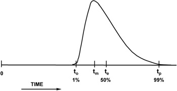
Figure 9-1: PERT estimates.
Originally, PERT analysis assumed a continuous Beta distribution of outcomes defined by these three parameters, similar to the graph in Figure 9-1. This distribution was chosen because it is relatively easy to work with in computer simulations and it can skew to the left (as in Figure 9-1) or to the right when the three estimating parameters are asymmetric. When it is symmetric, the Beta distribution is the Normal distribution (the Gaussian, bell-shaped curve).
PERT Time
PERT Time analysis using computer simulation takes these data and generates a random sample from the distribution associated with each project activity. These samples are then used as duration estimates to calculate the critical (longest) path through the network using standard critical path methodology (CPM) analysis. If PERT Time analysis were only done once, it would not be any more useful for risk analysis than CPM, but the PERT methodology repeats the process over and over, each time using new randomly generated activity duration estimates consistent with the chosen ranges. For each new schedule, CPM is used to calculate the project's critical path, and over many repetitions PERT builds a histogram of the results.
Current PERT and other computer modeling tools offer many alternatives to the Beta distribution. You may use Triangular, Normal, Poisson, and many other distributions, and with most software you can even enter histograms defining discrete estimates with associated probabilities. (For example, you may expect a 50 percent probability that the activity will complete in fifteen days, a 40 percent chance that it will complete in twenty days, and a 10 percent chance that it will complete in thirty days. These scenarios are generally based on probabilities associated with known risks for which incremental estimates are made—the five-day slip associated with a contributor who may need to take a week of leave to deal with a family situation, the fifteen-day slip associated with a problem that requires completely redoing of all the work).
As discussed in Chapter 7, the precise choice of the distribution shape is not terribly important, even for activity-level risk analysis. At the project level, it becomes even less relevant. The reason for this is that the probability density function for the summation of randomly generated samples of most types of statistical distributions (including all the realistic ones) always resembles a Normal, bell-shaped, Gaussian distribution. This is a consequence of the central limit theorem, well established by statisticians, and it is why the output of PERT analysis nearly always looks like a symmetric, bell-shaped curve. The Normal distribution has only two defining parameters, the mean and the variance (the square of the standard deviation). Early on with PERT, it was recognized that you could calculate these two parameters for the Beta distribution the activity estimates, using the formulas referenced earlier:
te = (to + 4tm + tp)/6, where
te is the "expected" duration—the mean
to is the "optimistic" duration
tm is the "most likely" duration
tp is the "pessimistic" duration
and
σ = (tp - to)/6, where
σ is the standard deviation
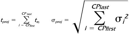
For many projects, the expected duration and standard deviation can be calculated for the project as a whole fairly easily. First, build a network of project activities using the calculated "expected" PERT durations for all estimates. Then, do a critical-path analysis to identify all critical activities. When there is a single, dominant critical path for the "expected" project, the expected duration for the project is the result you just generated—the sum of all the expected durations along the critical path. The standard deviation for the project, one measure of overall project risk, can be calculated from the estimated standard deviations for the same activities. PERT uses the following formulas:
Where
|
tproj |
= |
Expected project duration |
|
CPi |
= |
Critical path activity i |
|
tei |
= |
"Expected" CP estimate for activity i |
|
σproj |
= |
Project standard deviation |
|
σi2 |
= |
Variance for CP activity i |
These formulas work well whenever there is essentially only one critical path, or schedule failure mode, for the project. PERT gets more complicated when there are additional paths in the project that are roughly equivalent in length to the longest one. When this occurs, these formulas underestimate the expected project duration (it is actually slightly higher), and they overestimate the standard deviation. For project networks that have several "longest" paths, a full PERT analysis using computer simulation provides better results than the formulas. The reason these formulas are inaccurate was introduced in Chapter 4, in the discussion of multiple critical paths. There, the distinction between "Early/on time" and "Late" was a sharp one, with no allowance for degree. PERT analysis uses distributions for each activity and creates a spectrum of possible outcomes for the project, but the same logic—more failure modes lead to lowered success rates—is unavoidable. Since any of the parallel critical paths may end up being the longest for each simulated case, each of them contributes to the result for the project as a whole. The simple project considered in Chapter 4 had the network diagram in Figure 9-2, with one critical path across the top ("A-D-J") and a second critical path along the bottom ("C-H-L").
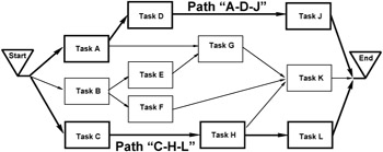
Figure 9-2: Project with two critical paths.
PERT analysis, as should be expected, shows that there is about one chance in four that the project will complete on time or earlier than the expected durations associated with each of the critical paths. The distribution of possible outcomes has about one-quarter of the left tail below the expected dates, and the peak and right tail are above it, similar to Figure 9-3. The resulting distribution is still basically bell-shaped, but, compared with the distributions expected for each critical path, it has a larger mean and is narrower (a smaller standard deviation).
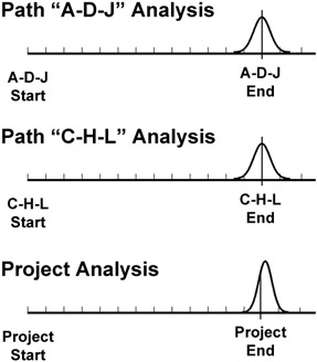
Figure 9-3: PERT results.
To consider this quantitatively, imagine a project plan using "50 percent" expected estimates that has a single dominant critical path of one hundred days (five months) and a standard deviation of five days. (If the distribution of expected outcomes is assumed symmetric, the PERT optimistic and pessimistic durations—plus or minus three standard deviations—would be roughly 85 days and 115 days, respectively). PERT analysis for the project says you should expect the project to complete in five months (or sooner) five times out of ten, and in five months plus one week over eight times out of ten (about five-sixths of the time)—pretty good odds.
If a second critical path of one hundred days is added to the project with similar estimated risk (a standard deviation of five days), the project expectation shifts to one chance in four of finishing in five months or sooner. (Actually, the results of the simulation based on one thousand runs shows 25.5 percent. The results of simulation should never be expected to match the theoretical answer exactly.) In the simulation, the average expected project duration is a little less than 103 days, and the similar "five-sixths" point is roughly 107 days. This is a small shift (about one-half week) for the expected project, but it is a very large shift in the probability of meeting the date that is printed on the project Gantt chart—from one chance in two to one chance in four.
Similar simulations for three and four parallel critical paths of equivalent expected duration and risk produce the results you would expect. For three paths of one hundred days, the project expectation falls to one chance in eight of completing on or before one hundred days (the simulation showed 13 percent) and an expected duration of roughly 104 days. The project with four failure modes has one chance in sixteen (6.3 percent in the model), and the mean for the project is a little bit more than 105 days. The resulting histogram for this case, based on 1,000 samples from each of four independent, Normally distributed parallel paths with a mean of one hundred days and a standard deviation of five days, is in Figure 9-4. (The jagged distribution is typical of simulation output.)
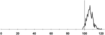
Figure 9-4: PERT histogram.
For these multiple critical path cases, the distribution mean increases, and the range compresses somewhat, reducing the expected standard deviation. The reason for this is that the upper data boundary for the analysis is unchanged, while each additional critical path tends to further limit the effective lower boundary. For the case in Figure 9-4, the project duration is always the longest of the four, and it becomes less and less likely that this maximum will be near the optimistic possibilities with each added path. Starting with a standard deviation for each path of five days, the resulting distribution for a project with two similar critical paths has a standard deviation of about 4.3 days. For three paths it is just under four days, and with four it falls to roughly 3.5 days, the statistic for the example in Figure 9-4. The resulting distributions also skew slightly to the left, for the same reasons; the data populating the histograms is being compressed, but only from the lower side.
PERT Cost
PERT analysis is most commonly performed for duration estimates, but it can also be used for effort and cost estimates. As with PERT Time, PERT Cost generates expected estimates for activities, as well as for the entire project. Unlike the PERT Time analysis, where only data from the calculated critical path are needed, PERT Cost sums the expected cost data and variance information from all project activities. Because of this, the formulas analogous to PERT Time for deriving project-level cost results are equivalent to simulation.
Using PERT
True PERT analysis software uses computer simulation, and for this reason the whole idea of PERT was impractical before the late 1950s. Starting then, simulations using Monte Carlo techniques began to be widely used to analyze many kinds of complex systems, including projects. Initially, PERT was very expensive (and slow), so it was undertaken only for the largest, most costly projects. This is no longer an issue with today's inexpensive desktop systems.
The issue of data quality for PERT analysis was also significant in early implementations, and this drawback persists. Generating range estimates remains difficult, especially when defined in terms of "percent tails," as is generally done in PERT literature. Considering that the initial single-point "most likely" estimate may not be very precise or reliable, the upper and lower boundary estimates are likely to be even worse. Since at least some of the input data are inexact, the "garbage in/garbage out" problem is a standard concern with PERT analysis.
This, added to the temptation to misuse the "optimistic" estimates by overeager managers and project sponsors, has made sustained use of PERT for technical projects difficult. This is unfortunate, because even if PERT analysis is applied only to suspected critical activities using manual approximations, it can still provide valuable insight into the level of project risk, and some methods require only modest additional effort. There are a number of approaches to PERT and PERT-like analysis, from manual approximations to full computer simulation. A summary of choices follows.
Manual PERT Approximation
One way to use PERT concepts is based on a technique discussed earlier. If you have a project scheduling tool, and project schedule information has been entered into the database, most of the necessary work is already done. The duration estimates in the database are a reasonable first approximation for the optimistic estimates, or the most likely estimates (or both). To get a sense of project risk, make a copy of the database (before you save it as a baseline), and enter new estimates for each activity where you have developed a worst-case or a pessimistic estimate. The Gantt chart based on these estimates will display end points for the project that are further out than the original schedule. By associating a Normal distribution with these points, a rough approximation of the output for a PERT analysis may be inferred.
The method used for scaling and positioning the bell-shaped curve can vary, but at least half of the distribution ought to fall between the lower "likely" boundary and the upper "pessimistic" limits defined by the end points of the two Gantt charts. Since it is very unlikely that all the things that could go wrong in the project will actually happen, the upper boundary should line up with a point several standard deviations from the mean, far out on the distribution tail. (Keep in mind, however, that none of your unknown project risk is yet accounted for.) The initial values in the scheduling database are probably somewhere below the mean of the distribution, though the exact placement should be a function of perceived accuracy for your estimates and how conservative or aggressive the estimates are. A histogram similar to Figure 9-5, using the initial plan as about the 20 percent point (roughly one standard deviation below the mean) and the worst-case plan to define the 99 percent point (roughly three standard deviations above the mean) is not a bad first approximation.
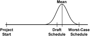
Figure 9-5: PERT approximation.
If the result represented by Figure 9-5 looks unrealistic, it may improve things if you calculate "expected" estimates, at least for the riskiest activities on or near a critical path. If you choose to do the arithmetic, a third copy of the database can be populated with "expected" estimates, defining the mean (the "50 percent" point) for the Normal distribution. The cumulative graph of project completion probabilities equivalent to Figure 9-5 looks like Figure 9-6.
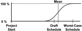
Figure 9-6: PERT estimates.
Although this sort of analysis is still subjective, the additional effort it requires is small once you generate a preliminary schedule for the project, and it provides valuable insight regarding project risk.
One of the most valuable things about analytical tools such as PERT is that they provide a very concrete, specific result. Either the results of a PERT analysis will look reasonable to you or they will seem "wrong." If the results seem realistic, they will probably be useful. If they look unrealistic, it usually indicates that additional work and planning are warranted. Odd PERT results are a good indication that your activity list is incomplete, your estimates are inaccurate, you missed some dependencies, you underestimated some risks, or your preliminary plan has some other defect.
Even this "quick and dirty" PERT approximation provides insight into the thoroughness of your project plan.
Using Computer Spreadsheets
Particularly for resource analysis, a computer spreadsheet such as Lotus 1-2-3 or Microsoft Excel is a very easy way to quickly assess three cost (or effort) estimates to derive an overall project-level budget analysis. A list of all the activities in one column with the "most likely" and range estimates in adjacent columns can be readily used to calculate expected estimates and variances for each activity and for the project as a whole. Using the PERT formulas for cost, it is simple to accumulate and evaluate data from all the project activities (not just from the critical path). The sum of all the expected costs and the calculated variance can be used as an approximation for PERT analysis of the project budget. Assuming a Normal distribution centered on the sum of the expected cost estimates with a spread defined by the calculated standard deviation shows the range that may be expected for project cost.
You could also generate "expected" duration estimates for the project by entering three duration estimates into the same spreadsheet. You can then use these "expected" duration estimates to locate your project critical path, either by manual inspection (for small projects) or by importing the data into a computer scheduling tool. If the "expected" project has a single, dominant critical path, the overall project PERT Time analysis may be derived with good accuracy, using the spreadsheet and the PERT formulas, but you must include only the activities associated with the longest path in your project network. The project PERT analysis generated this way is essentially similar to the manual approximation method discussed previously, with a Normal distribution centered on the sum of the expected duration estimates for the critical path and a spread defined by the calculated standard deviation.
For projects that have several paths roughly equal to the critical path, this method still may be used, but it will underestimate the expected project duration and overestimate the standard deviation.
Computer Scheduling Tools
True PERT analysis capability is not common in computer-based scheduling tools, and what is available tends to be implemented in quirky and mysterious ways. (This is not to be confused with the generating of "PERT" charts to display the network of project activities. All scheduling tools generate at least some rudimentary version of "PERT" charts. As discussed before, these charts are unrelated to PERT analysis and project risk.) This section mentions a number of scheduling tools, but it is far from exhaustive. Mention of a tool is not meant to imply that it is good, and nothing negative is implied about any tools that are omitted.
There are dozens of applications available for project scheduling, ranging from minimalist products that implement rudimentary activity analysis to high-end, Web-enabled enterprise applications. Often, families of software offering a range of capabilities are sold by the same company. Almost any of these tools may be used for determining the project critical path, but risk and PERT analysis using most of these tools, even some fairly expensive ones, often requires the manual processes discussed already or purchase of additional, specialized software (more on this specialized software follows).
Some rudimentary PERT analysis capability in scheduling software begins to show up in the midlevel products, which includes Microsoft Project, CA SuperProject, Scitor Project Scheduler, and other single-user products with prices comparable to home-office software. However, PERT capability in these products, if it is done at all, is based on calculations, not simulation.
For example, a very basic PERT capability was introduced into Microsoft Project 98 and continues in more current versions. It is possible to enter the three estimates into a "PERT Entry Sheet" and have the software use these data to calculate the duration estimates that are used in the database for the primary project Gantt chart. Except for the mislabeling of "most likely" as "expected" and then calling the calculated weighted average "estimated" instead of "expected," MS Project works much as it should for basic PERT schedule analysis. It even will generate optimistic, "most likely" (mislabeled "expected"), and pessimistic Gantt views for you to look at that are based on the three entered estimates, but it does not calculate an expected variance.
If you carefully read the descriptions of what the software does, and what data should be entered where, using MS Project and other similar software can be a convenient way to assemble project PERT data. Generating PERT results similar to the manual approximation and spreadsheet methods is not difficult, but only for schedule analysis. (Even basic project resource analysis is not a strong feature of midrange computer scheduling tools.)
High-end project management tools, which are both more capable and more costly than the ubiquitous midrange tools, frequently provide at least some built-in "what if?" capability for risk analysis. These products have more complex user interfaces, multiuser capability, and, consequently, steeper learning curves. Open-Plan Professional, from Welcom Software Technology, provides full integrated PERT analysis, and other high-end products, such as Primavera Enterprise and Project Workbench, from Niku, provide optional capabilities. Even with the high-end tools, though, PERT analysis requires an experienced project planner with a solid understanding of the process.
PERT Simulation Tools
Tools that provide true simulation-based PERT functionality are of two types. If you plan to implement full PERT capability, you will need either to locate PERT analysis software compatible with your project scheduling tool or to select a stand-alone PERT analysis application. Again, there are many, many options available in both of these categories; the examples mentioned are not endorsements, nor are omissions intended as criticism.
There are quite a few applications designed to provide simulation-based risk analysis that either integrate into high-end tools or "bolt on" to midrange scheduling packages. If such an add-on capability is available for the software you are using (or plan to use), you can do a PERT analysis without having to reenter or convert any of your project data. With the stand-alone software, project information must be input a second time or exported. Unless you also need to do some nonproject simulation analysis, add-on PERT analysis software is also generally a less expensive option.
Two tools that implement PERT directly for Microsoft Project are Risk+, from C/S Solutions, and @Risk, from Palisade Corporation. Each of these products offers similar capability at roughly the cost of a midrange scheduling tool. The exact functions offered and the user interface differ somewhat, but each product, even in its basic version, offers the necessary functions, operates with data entered into the MS Project database, and supports a number of reporting options.
Similar risk analysis software is available for the products in the Primavera suite, including its Monte Carlo add-on software. Other available project management tools also support partner-supplied PERT modules. The marketplace for these tools evolves rapidly, and versions (and even product names) change often, so it is a good idea to do some research before committing to specific risk management software to use with your scheduling tool.
Even if you are using scheduling software that can't perform PERT analysis, there are still ways to do it. The easiest solutions to implement are simulation applications specifically designed to do project schedule analysis. Data exported from MS Project and quite a few other scheduling tools can be used by tools such as Pertmaster Professional + Risk, from Pertmaster, Ltd., and Predict! Risk Analyser, from Risk Decisions, Ltd. These tools and others, including both Risk+ and @Risk, can also operate on data stored in computer spreadsheets. Exporting the data from a scheduling tool can be difficult the first time, but, once established, the process is fairly painless.
In addition to products specifically designed for PERT analysis, there are also general-purpose simulation applications that could be used, including decision-oriented software packages such as Crystal Ball, from Decisioneering Corporation, and Analytica, from Lumina Decision Systems, both of which are designed to interface with data in spreadsheets and other data formats. You can even perform PERT analysis using general-purpose statistical analysis software such as the SAS products from the SAS Institute, Minitab, from Minitab, Inc., and the SPSS products from SPSS, Inc. For the truly masochistic, it is even possible to do PERT analysis using only a spreadsheet—Microsoft Excel includes functions for generating random samples from various distribution types, as well as statistical analysis functions for interpreting the data.
Implementing PERT
As you can see, there are many methods for evaluating projects using PERT concepts. Some are quick and relatively easy to do and provide subjective but still useful insight into project risk. Other, more robust PERT methods offer very real risk management benefits, but they also carry costs, including investment in software, generation of more data, and increased effort. Before deciding to embark on a full-scale PERT analysis on a project, especially the first time, you must carefully consider the costs and added complexity.
A primary benefit of PERT analysis (shared to some degree with the approximate techniques discussed earlier) is the graphic and visible contrast between the deterministic-looking schedule generated by point-estimate critical path methods and the range of possible end points (and associated probabilities) that emerge from PERT analysis. The illusion of certainty fostered by single-estimate Gantt charts is inconsistent with the actual risk present in technical projects. The easy-to-see output from PERT analysis is a good antidote for excessive project optimism.
In addition, PERT tools that use Monte Carlo simulation techniques are able to display project schedules more realistically in cases where the project has more than one critical (or very nearcritical) path, and some PERT analysis tools even provide for project branching and "decision-tree" type analysis. Project scheduling tools assume that all choices and decisions can be made during planning and cemented into an unchanging project plan, which is not very realistic for most technical projects.
All this benefit from using PERT is far from free. (In projects there are always trade-offs.) For one thing, it can be a lot of work, and generating realistic input data forces project staff members to do even more of the sort of analysis that they already dislike doing. PERT analysis, like most analytical methodologies, can generate extremely precise-looking output, creating an illusion of precision. The actual precision of the output generated can never be any better than that of the least accurate inputs. Rounding the results off to whole days is about the best you can expect, yet results with many decimal places are reported by some software. This illusion of precision is particularly ironic considering the quality of typical project input data. Generating useful estimates and the effort of collecting, entering, and interpreting PERT information represent quite a bit of work.
In project environments that currently lack systematic project-level risk analysis, it may be prudent to begin with a modest PERT effort on a few projects and expand as necessary for future projects.
Other Project Modeling and Decision Support
Project risk analysis also includes decision making. There are many techniques for decision making, varying from informal examination of small decisions to elaborate processes used in complex, difficult situations. One frequently used technique employs decision trees, discussed in Chapter 7. When they are simple, these branching diagrams are not difficult to evaluate through inspection. As decisions get more complicated, there are software applications and more analytical techniques available. Some decisions also benefit from more elaborate analysis, using the same simulation and statistical methods used for full-scale PERT-type project analysis. There are many computer tools available for decision modeling and analysis.
Decision-Making Process
Good decisions result from systematic group dialogue to reach agreement on one choice among a set of alternatives. More consistent decisions result from an organized process with sufficient formality to ensure thoroughness and broad participation. The overall process includes:
- Defining the issue or question requiring a decision
- Determining how, and when, and by whom the decision will be made
- Forming options and selecting decision criteria
- Analyzing options and making the decision
The first step in the decision process is to clearly define the issue requiring a decision. To avoid jumping into problem-solving mode too quickly, you should initially focus on the question "What problem are we solving?" Use root cause analysis to understand the underlying source of the issue, not just the obvious symptoms. If clarification of the overall problem proves impossible, decompose it into smaller, more tractable subproblems. Frame the issue by identifying how the decision will be used, and summarize the issue in a concise statement.
Effective decision making requires participation by the right people. Involve people who will be affected by the decision, as well as those who will need to approve the choice that you make. Also, identify the experience, knowledge, and skills required for a good decision, and get commitment from qualified people to participate in the decision-making process.
While some decisions must be made quickly, with very little discussion or group input involved, other decisions require consensus, or even unanimity. Determine how you will arrive at a decision, and gain support for your process. Set a deadline for the decision that will allow adequate time for discussion and analysis.
Once you have determined the issue and how to proceed, develop a set of options or alternative solutions for the problem statement, using methods such as brainstorming, cause-and-effect diagrams, root cause analysis, and creative problem solving. Also, identify any criteria that are important for the decision. Define measurable criteria and prioritize them by relative importance. Evaluation criteria could include factors such as speed, cost, total required effort, and the number of people involved. Discussing the criteria and their relative weights improves understanding of the issue and leads to group buy-in for the decision.
You can evaluate simple decisions using a "pros and cons" list or a simple matrix with weighted decision criteria. For more complex situations, spreadsheets or software tools may help with your evaluation. However you evaluate your potential options, use the information to prioritize the alternatives. Discuss the top several items; if there are people who believe that the top item is not the best choice, explore why. Whenever an analytical process results in the "wrong" answer, it may indicate that your assumptions or data are faulty. Your criteria, weights, or evaluations may need adjustment, or you may need further discussion to develop consensus. Before adopting any of the alternatives, check for any unintended consequences or risks.
When you reach agreement, stop the discussion. Verify support for the decision among all those involved, communicate your decision, and put it into action.
Decision Support Software
As with project analysis tools, there is no dearth of computer applications to help with decision making. Some software available is related to the PERT tools already discussed, such as Precision Trees, from Palisade Corporation, the same company that offers the @Risk application. Other tools for decision-tree analysis include DPL, from Applied Decision Analysis, and DATA, from Treeage Software. There are also a number of packages that support implementation of the matrix-oriented analytical hierarchy process, including Expert Choice, from Expert Choice, Inc., but evaluating decisions using a matrix of evaluations of weighted criteria is not that complicated for many decisions, whether done manually or using a computer spreadsheet.
Several of the simulation-support tools discussed for PERT analysis are also useful for analyzing decisions, such as Crystal Ball, from Decisioneering Corporation, and Analytica, from Lumina Decision Systems. Simulation capability allows deeper exploration of the range of possible outcomes from decisions, which can be valuable in evaluating very complex decisions.
Analysis of Scale
Quantitative project analysis using all the preceding techniques, either with computer tools or using manual methods, is based on details of the project work—activities, decisions, worst cases, resource issues, and other planning data. It is also possible to assess risk on the basis of the overall size of the project, because the overall level of effort is another important risk factor. Projects only 20 percent larger than previous work represent significant risk.
Scale analysis is based on the overall effort that the project plan calls for. Projects fall into three categories—low risk, normal risk, and high risk—determined by the anticipated effort as compared with earlier, successful projects. Scale assessment begins by accumulating the data from the bottom-up project plan to determine total project effort, measured in a suitable unit such as "effort-months." The calculated project scale can then be compared with the effort actually used on several recent, similar projects. In selecting comparison projects, look for work that had similar deliverables, timing, and staffing so that the comparison will be as valid as possible. If the data for the other projects are not in the form you need, do a rough estimate using staffing levels and project duration. If there were periods in the comparison projects where significant overtime was used, especially at the end, account for that effort, as well. The numbers generated do not need to be exact, but they do need to fairly represent the amount of overall effort actually required to complete the comparison projects.
Using the total of planned effort-months for your project and an average from the comparison projects, determine the risk:
|
Low risk |
Less than 60 percent of the average |
|
Normal risk |
Between 60 percent and 120 percent of the average |
|
High risk |
Greater than 120 percent of the average |
These ranges center on 90 percent rather than 100 percent because the comparison is between actual past project data, which include all changes and risks that occurred, and the current project plans, which do not. Risk arises from other factors in addition to size, so consider raising the risk assessment one category if:
- The schedule is significantly compressed
- The project requires new technology
- 40 percent of the project resources are either external or unknown
Project Appraisal
Scale analysis can be taken a further step, both to validate the project plan and to get a more precise estimate of risk. The technique requires an "appraisal," similar to the process used whenever you need to know the value of something, such as a piece of property or jewelry, but you do not want to sell it to find out. Value appraisals are based on the recent sale of several similar items, with appropriate additions and deductions to account for small differences. If you want to know the value of your home, an appraiser examines it and finds descriptions of several comparable homes recently sold nearby. If the comparison home has an extra bathroom, a small deduction is made to its purchase price; if your house has a larger, more modern kitchen, the appraiser makes a small positive adjustment. The process continues, using at least two other homes, until all factors normally included are assessed. The average adjusted price that results is taken to be the value of your home—the current price for which you could probably sell it.
The same process can be applied to projects, since you face an analogous situation. You would like to know how much effort a project will require, but you are not in a position to execute all the work to find out. The comparisons in this case are two or three recently completed similar projects, for which you can ascertain the number of effort-months that were required for each. (This starts with the same data the scale analysis technique uses.)
From your bottom-up plan, calculate the number of effort-months your project is expected to take. The current project can be compared to the comparison projects, using a list of factors germane to your work. Factors relevant to the scope, schedule, and resources for the projects can be compared, as in Figure 9-7 (which was quickly assembled using a computer spreadsheet).
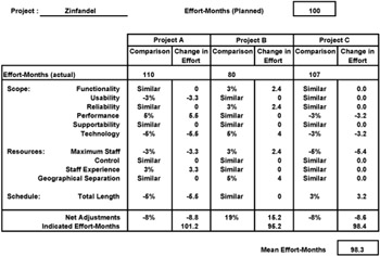
Figure 9-7: Project appraisal.
One goal of this technique is to find comparison projects that are as similar as possible so that the adjustments will be small and the appraisal can be as accurate as possible. If a factor seems "similar," no adjustment is made. When there are differences, adjust conservatively, such as:
|
Small differences |
Plus or minus 2–5 percent |
|
Larger differences |
Plus or minus 7–10 percent |
The adjustments are positive if the current project has the higher risk and negative if the comparison project seems more challenging.
The first thing you can use a project appraisal for is to test whether your preliminary plan is realistic. Whenever the adjusted comparison projects average to a higher number of effort-months than your current planning shows, your plan is almost certainly missing something. Whenever the appraisal indicates a difference greater than about 10 percent compared with the bottom-up planning, work to understand why. What have you overlooked? Where are your estimates too optimistic? What activities have you not captured? Also, compare project appraisal effort-month estimates with the resource goal in the original project objective. A project appraisal also provides early warning of potential budget problems.
One reason project appraisals are generally larger than the corresponding plan is risk. The finished projects include the consequences of all risks, including those that were invisible early in the work. The current project planning includes only data on the known risks for which you have incorporated risk prevention strategies. At least part of the difference between your plan and an appraisal results from the comparison projects' "unknown" risks, contingency plans, and other risk response efforts.
In addition to plan reviews, project appraisals are also useful in project-level risk management. Whenever there is a major difference between the parameters of the planned project and the goals stated in the project objective, the appraisal shows why this is so, convincingly and in a very concise format. A project appraisal is a very effective way to begin discussion of options and trade-offs with the project sponsor, which is addressed in Chapter 10.
Project Metrics
Project measurement is essential to risk management. It also provides the historical basis for other project planning and management processes, such as estimation, scheduling, controlling, and resource planning. Metrics drive behavior, so selecting appropriate factors to measure can have a significant effect on motivation and project progress. Bill Hewlett, a founder of HP, was fond of saying, "What gets measured gets done." Metrics provide the information needed to improve processes and to detect when it is time to modify or replace an existing process. Established metrics also are the foundation of project tracking, establishing the baseline for measuring progress. Defining, implementing, and interpreting a system of ongoing measures is not difficult, so it is unfortunate that on many projects these steps either are not done at all or are done poorly.
Establishing Metrics
Before deciding what to measure, carefully define the behavior you want and determine what measurements will be most likely encourage that behavior. Next, establish a baseline by collecting enough data to determine current performance for what you plan to measure. Going forward, you can use metrics to detect changes, trigger process improvements, evaluate process modifications, and make performance and progress visible.
The process begins with defining the results or behavior you desire. For metrics in support of better project risk management, a typical goal might be "Reduce unanticipated project effort" or "Improve the accuracy of project estimates." Consider what you might be able to measure that relates to the desired outcome. For unanticipated project effort, you might measure "total effort actually consumed by the project versus effort planned." For estimation accuracy, a possible metric might be "cumulative difference between project estimates and project results, as measured at the project conclusion."
Metrics are of three basic types: predictive, diagnostic, and retrospective. An effective system of metrics generally includes measures of more than one type, providing for good balance.
- Predictive metrics use current information to provide insight into future conditions. Because predictive metrics are based on speculative rather than empirical data, they are typically the least reliable of the three types. Predictive metrics include the initial assessment of project "return on investment," the output from the quantitative risk management tools, and most other measurements based on planning data.
- Diagnostic metrics are designed to provide current information about a system. On the basis of the latest data, they assess the state of a running process and may detect anomalies or forecast future problems. The unanticipated effort metric suggested before is based on earned value, a useful diagnostic project metric.
- Retrospective metrics report after the fact on how the process worked. Backward-looking metrics report on the overall health of the process and are useful in tracking trends. The estimating accuracy example already mentioned is based on the estimating quality factor metric as defined by Tom DeMarco, a retrospective metric discussed in more detail later in this chapter.
Measuring Projects
The following section includes a number of useful project metrics. No project needs to collect all of them, but one or more measurements of each type of metric, collected and evaluated for all projects in an organization, can significantly improve the planning and risk management on future projects. These metrics relate directly to projects and project management. A discussion of additional metrics, related to financial measures, follows this section.
When implementing any set of metrics, you need to spend some time collecting data to validate a baseline for the measurements before you make any decisions or changes. Until you have a validated baseline, measurements will be hard to interpret, and you will not be able to determine the effects of process modifications that you make. There is more discussion on selecting and using metrics in Chapter 10.
Predictive Project Metrics
Most predictive project metrics relate to factors that can be calculated using data from your project plan. These metrics are fairly easy to define and calculate, and they can be validated against corresponding actual data at the project close. Over time, the goal for each of these should be to drive the predictive measures and the retrospective results into closer and closer agreement. Measurement baselines are set using project goals and planning data.
Predictive metrics are also useful in helping you anticipate potential project problems. One method of doing this is to identify any of these predictive metrics that is significantly larger than typically measured for past, successful projects—a variance of 15 to 20 percent represents significant project risk. (The first metric, "total effort," is the basis for the "project scale" risk assessment discussed earlier in the chapter.) A second use for these metrics is to correlate them with other project properties. After measuring factors such as unanticipated effort, unforeseen risks, and project delays for ten or more projects, some of these factors may reveal sufficient correlation to predict problems with fair accuracy.
Some predictive project metrics include:
- Total project effort: effort-month total for all project activities.
- Budget at completion (BAC): the monetary equivalent of total project effort. This metric is associated with project earned value analysis.
- Project appraisal: the expected total project effort based on comparisons with completed similar projects, adjusting for significant differences.
- Project complexity index: the sum of several deliverable related factors, multiplied by a scale factor (described in Chapter 3).
- Aggregated schedule risk: the sum of all project slippage expected, based on using contingency plans and weighted by probability of use.
- Aggregated budget risk: the sum of all additional project costs expected, based on using contingency plans and weighted by probability of use.
- Survey-based risk assessment score: collaborative accumulation of risk data from project staff using a customized set of assessment questions.
- Logical project length: the maximum number of distinct activities on any network path.
- Logical project width: the maximum number of parallel activities found in the project network.
- Logical project complexity: the ratio of activity dependencies to activities.
- Project independence: the ratio of internal activity dependencies to all dependencies.
- Project staffing: maximum number of project staff.
- Sum of activity durations: total duration of all activities if executed sequentially.
- Sum of total activity float: total float (or slack) accumulated from all planned activities.
- Project density: the ratio of the sum of activity durations to the sum of activity durations plus the sum of total activity float.
Diagnostic Project Metrics
Diagnostic metrics are based on measurements taken throughout the project, and they are used to detect adverse project variances and project problems, either in advance or as soon as is practical. Measurement baselines are generally set using a combination of stated goals and historical data from earlier projects. Diagnostic metrics are comparative measures, either trend-oriented (comparing the current measure with earlier measures) or prediction-oriented (comparing measurements with corresponding predictions, generally based on planning).
A large family of diagnostic project metrics relates to the concept of earned value analysis (EVA). This technique for project measurement and control begins with allocating the portion of the project budget associated with project activities (the costs associated with effort) to each of the planned project activities. The sum of all these allocated bits must exactly equal 100 percent of the project staffing budget. As the project executes, EVA collects data on actual costs and actual timing for all completed activities so that ratios and differences may be calculated. The definitions for these diagnostic metrics follow, stated in financial terms. The mathematics of EVA are identical for equivalent metrics that are based on effort data (person-hours planned versus person-hours actually consumed), and a parallel set of metrics defined this way are sometimes used. The terminology for earned value analysis was changed in the PMBOK Guide, 2000 edition, but both the new and the still commonly used older terminology are included here.
Like PERT analysis, the value of EVA for technical projects is the subject of much discussion. It can represent quite a bit of overhead, and, for many types of technical projects, tracking data at the level required by EVA is thought to be overkill. If the metrics for EVA seem impractical, the related alternative of activity closure index, which provides similar diagnostic information on the basis of the higher granularity of whole activities, provides similar information with a lot less effort. EVA typically can accurately predict project overrun at the point where 15 percent of the project staffing budget is consumed. Activity closure rate is less precise, but even it will accurately spot an overrun trend well before the project halfway point.
Some diagnostic project metrics include:
- Earned value (EV), or budgeted cost of work performed (BCWP): a running accumulation of the costs that were planned for every project activity that is currently complete. The terms are synonymous, but EV is currently preferred in the PMBOK Guide.
- Actual cost (AC), or actual cost of work performed (ACWP):a running accumulation of the actual costs for every project activity that is currently complete. The terms are synonymous, but AC is currently preferred in the PMBOK Guide.
- Planned value (PV), or budgeted cost of work scheduled (BCWS): a running accumulation of the planned costs for every project activity that was expected to be complete up to the current time. The terms are synonymous, but PV is currently preferred in the PMBOK Guide. (PV is really a predictive project metric, because all the values for the whole project may be calculated from the baseline plan as an ever increasing amount of money. PV starts at zero, and at the project end it is equal to the budget at completion. PV may be treated as a diagnostic metric for earned value analysis, calculated periodically along with EV and AC.)
- Cost performance index (CPI): the ratio of earned value to actual cost. This ratio is the primary diagnostic metric used for EVA. When it is one or higher, the project is spending money (or equivalently, effort) at a rate that is equal to or less than the planned rate. When it is less than one, the "burn rate" for the project is too high, and it indicates a possible project budget overrun.
- Schedule performance index (SPI): the ratio of earned value to planned value. This ratio may be used to predict schedule problems, providing that resource use throughout the project is relatively constant. If resource use varies with project timing, SPI has limited usefulness.
- Cost variance (CV): the difference between earned value and actual cost, a measurement of how much the project is over or under budget. A cost variance percentage may be calculated as a ratio of CV to earned value. The CV percentage reports the current budget variance as a fraction. CV, like CPI, may be used to predict project overrun.
- Schedule variance (SV): the difference between earned value and planned value. Like the SPI metric, this absolute monetary difference is of value only if resource use is flat over time. Schedule variance percentage, the ratio of SV to earned value, presents the same information as a fraction.
- Activity closure index: the ratio of activities closed in the project so far to the number expected based on a linear extrapolation—in other words, for an N-week project, 1/N of the total number of activities per week. For example, by week six of a thirty-six-week project with 200 planned activities, roughly thirty-three activities should be complete. If only thirty are closed, the ratio is .9, indicating a potential schedule problem. This is a less complex, and less precise, variation on earned value analysis.
- Cumulative slip: the running sum for all activities of early schedule finish date minus actual activity completion date.
- Risk closure index: the ratio of risks closed (avoided, encountered, or otherwise no longer a risk) in the project divided by the number expected on the basis of a linear extrapolation.
Retrospective Project Metrics
Retrospective metrics are backward-looking and may be assessed only at the close of a project. Measurement baselines are based on prior history, and these metrics are most useful for longer-term process improvement.
Some retrospective project metrics include:
- Estimation quality factor (EQF): the ratio of project cost multiplied by duration, divided by an accumulated estimating error factor
- Performance to planned schedule: a variance measured in workdays or as a percentage of the planned schedule
- Performance to planned budget: a variance measured in financial terms or as a percentage of the planned budget
- Life-cycle phase effort percentages (for your life cycle)
- Testing effort as a percent of total project effort
- Performance to standard estimates for required or standardized project activities
The first metric listed, EQF, requires some explanation. Introduced in Controlling Software Projects by Tom DeMarco, EQF is a measure of how quickly erroneous estimates are detected and corrected. It is a unitless ratio based on the actual project duration multiplied by the actual project cost, divided by an accumulated estimating error factor. The estimating error factor is accumulated for the project by summing over the whole project the absolute value of the difference between the project cost estimate and the final project cost, multiplied by the amount of time the estimate was believed accurate. If the estimate was changed several times, the estimating error factor will be a number of these products, added together.
EQF sounds harder to calculate than it is, and it is evaluated only once per project. A graph with the project duration on the X axis and project budget on the Y axis defines a rectangle (as shown in Figure 9-8), the area of which is the numerator for EQF. The plot of cost estimates by date throughout the project defines a series of rectangles that share either a top or a bottom border with the larger rectangle that defines the numerator. The areas of all the smaller rectangles (shaded in the figure) added together are the denominator for EQF.
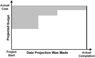
Figure 9-8: EQF example.
If the initial project cost estimate is exactly right and never changed, EQF is infinite, because you are dividing by an estimating error factor of zero. If the cost estimate starts at zero and stays there through the entire project, EQF is one, which is the effective minimum. (EQF lower than one is possible, but only for projects that begin with enormously padded budgets.) A project that increases the estimate linearly once a week until the project is done has an EQF of two, equal to a project that estimates the cost at one half the final figure and never changes it.
Figure 9-8 shows an EQF of roughly four (the grey area is about one quarter of the larger rectangle). This is about where one R&D lab at Hewlett-Packard started when it calculated EQF for several completed projects. Over a period of about a year, the average project in the lab improved to an EQF of almost 20, representing a typical overall estimating error of about 5 percent—very respectable. What gets measured gets done.
Financial Metrics
Project risk extends beyond the normal limits of project management, and project teams must consider and do what they can to manage risks that are not strictly "project management." There are a number of methods and principles used to develop predictive metrics that relate to the broad concept of return on investment (ROI), and an understanding of these is essential to many types of technical projects. As discussed in Chapter 3 with market risks, ROI analysis falls only partially within project management's traditional boundaries. Each of the several ways to measure ROI comes with benefits, drawbacks, and challenges.
The Time Value of Money
The foundation of most ROI metrics is the concept of the time value of money. This is the idea that a quantity of money today is worth more than the same quantity of money at some time in the future. How much more depends on a rate of interest (or discount rate) and the amount of time. The formula for this is:
PV = FV/(1 + i)n, where
PV is present value
FV is future value
i is the periodic interest rate
n is the number of periods
If the interest rate is 5 percent per year (.05) and the time is one year, $1 today is equivalent to $1.05 in the future.
Payback Analysis
Even armed with the time-value-of-money formula, it is rarely easy to determine the worth of any complex investment with precision, and this is especially true for investments in projects. Project analysis involves many (perhaps hundreds) of parameters and values, multiple periods, and possibly several interest rates. Estimating all of these data, particularly the value of the project deliverable after the completion of the project, can be very difficult.
The most basic ROI model for projects is simple payback analysis, which assumes no time value for money (equivalent to an interest rate of zero). This type of ROI metric has many names, including break-even time, payback period, or the "return map." Payback analysis adds up all expected project expenses and then proceeds to add expected revenues, profits, or accrued benefits, period by period, until the value of the benefits balances the costs. As projects rarely generate benefits before completion, the cumulative financials swing heavily negative, and it takes many periods after the revenues and benefits begin to reach "break even."
The project in the graph in Figure 9-9 runs for about five months, with a budget of almost $500,000. It takes another six months, roughly, to generate returns equal to the project's expenses. Simple payback analysis works fairly well for comparing similar-length projects to find the one (or ones) that recover their costs most rapidly. It has the advantage of simplicity, using predictive project cost metrics for the expense data and sales or other revenue forecasts for the rest.
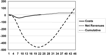
Figure 9-9: Simple payback analysis.
Refining simple payback analysis to incorporate interest (or discount) rates is not difficult. The first step is to determine an appropriate interest rate. Some analyses use the prevailing cost of borrowing money, others use a rate of interest available from external investments, and still others use rates based on business targets. The rate of interest selected can make a significant difference when evaluating ROI metrics.
Once an appropriate interest rate is selected, each of the expense and revenue estimates can be discounted back to an equivalent present value before it is summed. The discounted payback or break-even point again occurs when the sum, in this case the cumulative present value, reaches zero. For a nonzero interest rate, the amount of time required for payback will be significantly longer than with the simple analysis, since the farther in the future the revenues are generated, the less they contribute because of the time value of money. Discounted payback analysis is still relatively easy to evaluate, and it is more suitable for comparing projects that have different durations.
Payback analysis, with and without consideration of the time value of money, is often criticized for being too short-term. These metrics determine only the time required to recover the initial investment. They do not consider any benefits that might occur following the break-even point, so a project that breaks even quickly and then generates no further benefits would rank higher than a project that takes longer to return the investment but represents a much longer, larger stream of subsequent revenues or benefits.
Net Present Value
Total net present value (NPV) is another method to measure project ROI. NPV follows the same process as the discounted payback analysis, but it does not stop at the break-even point. NPV includes all the costs and all the anticipated benefits throughout the expected life of the project deliverable. Once all the project costs and returns have been estimated and discounted to the present, the sum represents the total present value for the project. This total NPV can be used to compare possible projects, even projects with very different financial profiles and time scales, basing the analysis on all expected project benefits.
Total NPV effectively determines the overall expected return for a project, but it tends to favor large projects over smaller ones, without regard to other factors. A related idea for comparing projects normalizes their financial magnitudes by calculating a profitability index (PI). The PI is a ratio, the sum of all the discounted revenues divided by the sum of all the discounted costs. PI is always greater than one for projects that have a positive NPV, and the higher the PI is above one, the more profitable the project is expected to be.
Even though these metrics require additional data—estimates of the revenues or benefits throughout the useful life of the deliverable—they are still relatively easy to evaluate.
Internal Rate of Return
Another way to contrast projects of different sizes is to calculate an internal rate of return (IRR). IRR uses the same estimates for costs and returns required to calculate total net present value, but, instead of assuming an interest rate and calculating the present value for the project, IRR sets the present value equal to zero and then solves for the required interest rate. Mathematically, IRR is the most complex ROI metric, as it must be determined using iteration and "trial and error." For sufficiently complicated cash flows, there may even be several values possible for IRR (this occurs only if there are several reversals of sign in the cash flows, so it rarely happens in project analysis). These days, use of a computer (or even a financial calculator) makes determining IRR fairly straightforward, if good estimates for costs and revenues are available. For each project, the interest rate you calculate shows how effective the project is expected to be as an investment.
ROI Estimates
All of these ROI methods are attempts to determine the "goodness" of financial investments, in this case, projects. Theoretically, any of these methods is an effective way to select a few promising projects out of many possibilities or to compare projects with other investment opportunities.
Due to their differing assumptions, these methods may generate inconsistent ranking results for a list of potential projects, but this is rarely the biggest issue with ROI metrics. In most cases, the larger, more fundamental problem is with input data. Each of these methods generates a precise numeric result for a given project that is based on the data. For many projects, this information comes from two sources that are historically not very reliable: project planning data and sales forecasts. Project planning data can be made more accurate over time using metrics and adjustments for risk, at least in theory. Unfortunately, project ROI calculations are generally made before much planning is done, when the project cost data are still based on vague information, or the estimates come from top-down budget goals that are not correlated with planning at all.
Estimates of financial return are an even larger problem. These estimates are not only usually very uncertain (based on sales projections or other speculative forecasts) but also much larger numbers, so they are more significant in the calculations. For product development projects, in many cases revenue estimates are higher by an order of magnitude or more, so even small estimating errors can result in large ROI variances.
ROI metrics can be very accurate and useful when calculated retrospectively using historical data, long after projects have completed. The predictive value of ROI measures calculated in advance of projects can never be any more trustworthy than the input data, so a great deal of variation can occur.
Key Ideas for Project Risk Analysis
- Survey contributors and stakeholders for risk assessments.
- Use worst-case estimates, contingency plan data, or PERT analysis to determine project uncertainty.
- Estimate project scale in effort-months.
Panama Canal Overall Risks (1907)
When John Stevens first arrived in Panama, he found a lack of progress and an even greater lack of enthusiasm. He commented, "There are three diseases in Panama. They are yellow fever, malaria, and cold feet; and the greatest of these is cold feet." For the first two, he set Dr. William Gorgas to work, and these risks were soon all but eliminated from the project.
For the "cold feet," Stevens himself provided the cure. His intense planning effort and thorough analysis converted the seemingly impossible into small, realistic steps that showed that the work was feasible; the ways and means for getting the work done were documented and credible. Even though there were still many specific problems and risks on the project, Stevens had demonstrated that the overall project was truly possible. This was quite a turnaround from John Wallace's belief that the canal venture was a huge mistake.
With Stevens's plan, nearly every part of the job relied on techniques that were in use elsewhere, and almost all the work required had been done somewhere before. Project funding was guaranteed by the U.S. government. There were thousands of people able, and very willing, to work on the project, so labor was never an issue. The rights and other legal needs were not a problem, especially after Theodore Roosevelt manipulated the politics in both the United States and in Panama to secure them. What continued to make the canal project exceptional was its enormous scale. As Stevens said, "There is no element of mystery involved; the problem is one of magnitude and not miracles."
Planning and a credible understanding of overall project risk are what convert the need for magic and miracles (which no one can confidently promise to deliver) into the merely difficult. Projects that are seen as difficult but possible are the ones that succeed; a belief that a project can be completed is an important factor in how hard and how well people work. When it looks as though miracles will be necessary, people tend to give up, and their skepticism may very well make the project impossible.
Introduction
- Why Project Risk Management?
- Planning for Risk Management
- Identifying Project Scope Risk
- Identifying Project Schedule Risk
- Identifying Project Resource Risk
- Managing Project Constraints and Documenting Risks
- Quantifying and Analyzing Activity Risks
- Managing Activity Risks
- Quantifying and Analyzing Project Risk
- Managing Project Risk
- Monitoring and Controlling Risky Projects
- Closing Projects
- Conclusion
- Appendix A Selected Detail From the PERIL Database
EAN: 2147483647
Pages: 130
