Hack 16. How Big Is the World?

If you wanted to make your own Google Maps server, how much hard drive space would you need?

Google Maps renders maps by stitching small images together. We seek to discover the storage capacity of such an image repository. By capturing and examining screenshots of Google Maps in action, we can estimate the map scale at each zoom level, which will give us an idea of how much space is necessary to store all the tiles for that zoom level. Finally, we can add the storage requirements for each zoom level and apply some simple rules of thumb to arrive at an idea of how much hard drive space is necessary to support a web mapping service such as Google Maps.

2.8.1. Economies of Scale

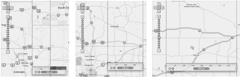
First, we need to discover the scaling factors used at each of the fifteen zoom steps. To accomplish this analysis, we use a tool called Art Director's Toolkit, which comes bundled with Mac OS X and which offers an overlay desktop ruler image for measuring pixel distances onscreen. In zoom levels 0 to 6, we measure the pixel length between the northeast corner of Colorado and the southeast corner of Wyoming. This distance is clearly marked on the map as a horizontal line, which makes measuring it easy. Figure 2-16 depicts zoom levels 0, 1, and 2, where the distances in question are 12, 24, and 48 pixels, respectively.

Figure 2-16. Zoom levels 0 through 2

In Figure 2-17, we see that, for zoom levels 3, 4, and 5, the same distances are 98, 196, and 394 pixels.

For zoom level 6, the distance between the northeast corner of Colorado and the southeast corner of Wyoming measures out at 790 pixels. Zoom level 7 was skipped because there was nothing to measure for itsmaller things were too small, and bigger things were too big. (Skipping it did not negatively impact the analysis.)

Figure 2-17. Zoom levels 3 through 5

In zoom levels 8 through 14, we measure the pixel length of the path from the intersection of Trenton Street and East 16th Avenue to the intersection of Verbena Street and East 16th Avenue in Denver, Colorado, which is within the metropolitan area closest to our previous locations. For zoom level 8, the distance is 9 pixels. For zoom levels 9, 10, and 11, the distances are 19, 37, and 74 pixels. The results are shown in Figure 2-18.

Figure 2-18. Zoom levels 8 through 11

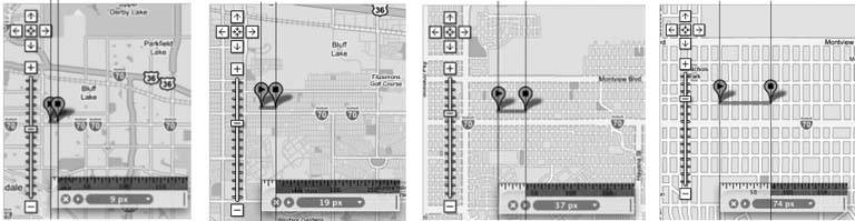
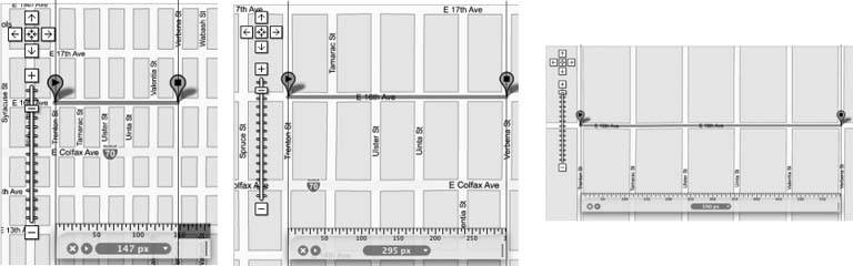
For zoom levels 12, 13, and 14, the distances are 147, 295, and 590 pixels. Figure 2-19 depicts this measurement.

Figure 2-19. Zoom levels 12 through 14

Now we can take the information from these measurements, and attempt to establish the numeric scale ratio between one zoom level and the previous one. Figure 2-20 presents the same relationships in three nicely formatted line graphs and Table 2-1 summarizes the data we collected.

Figure 2-20. Length ratios visualized in a series of line graphs

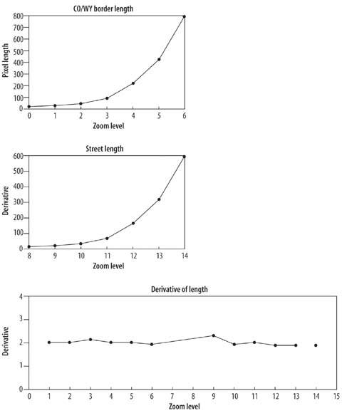
The conclusion we draw is that we can be fairly certain that the scale doubles with every increment of the zoom bar.

Table 2-1. Length ratios from one zoom level to the previous zoom level

Zoom	State border length	Ratio	Zoom	Street length	Ratio
0	12	n/a	8	8	n/a
1	24	2	9	19	2.38
2	48	2	10	37	1.95
3	98	2.04	11	74	2
4	196	2	12	147	1.99
5	394	2	13	295	2.01
6	790	2.01	14	590	2

 

2.8.2. So, How Much?

By zooming almost all the way out in Google Maps, we see that North America fits nicely in a 600 x 800pixel rectangular region, amounting to 480,000 pixels. Armed with this approximation, we proceed to estimate the pixel-area of this body at each zoom level. Table 2-2 depicts these relationships.

Table 2-2. Approximate area in pixels of North America for each zoom level

Zoom	Scale	Width	Height	Area in pixels
0	1	800	600	480,000
1	2	1,600	1,200	1,920,000
2	4	3,200	2,400	7,680,000
3	8	6,400	4,800	30,720,000
4	16	12,800	9,600	122,880,000
5	32	25,600	19,200	491,520,000
6	64	51,200	38,400	1,966,080,000
7	128	102,400	76,800	7,864,320,000
8	256	204,800	153,600	31,457,280,000
9	512	409,600	307,200	125,829,120,000
10	1,024	819,200	614,400	503,316,480,000
11	2,048	1,638,400	1,228,800	2,013,265,920,000
12	4,096	3,276,800	2,457,600	8,053,063,680,000
13	8,192	6,553,600	4,915,200	32,212,254,720,000
14	16,384	13,107,200	9,830,400	128,849,018,880,000

If we add up the areas, we find that 171,798,691,680,000 (171 trillion) pixels are needed to store all the bitmap information. Since all maps are made up of 256 x 256 tiles, one can venture to guess that there are 171,798,691,680,000 ÷ (256 x 256) = 2,621,439,997 (2.6 billion) potential tile files.

The color histogram of the maps in Figure 2-19 shows that about 60 percent of it is water. Assuming that Google observes such statistics, we guess that a single tile is used for all water regions. There are also lots of regions (such as tundra, deserts, and forests) where uniformly colored tiles can be used. Computing this accurately is difficult, but we will say it amounts to 10 percentof the data. So, only 30 to 40 percent of the tiles have unique data on them. This reduces the amount of data to 50 to 70 trillion raw data pixels stored in 750 million to 1 billion image files. Assuming a modest 1 byte per 6 pixels compression ratio (for LZW-encoded GIF format images), the storage required might be 50 to 70 trillion pixels * (1 byte/6 pixels) = 8 to 11 terabytes. If we consider that Google supports three map types at present (Map, Satellite, and Hybrid), this suggests that 24 to 33 terabytes are needed to store all the image data.

2.8.3. What About the Rest of the World?

Since we did our original analysis, Google Maps UK, Google Maps Japan, and Google Earth were introduced, providing further evidence of a lofty goal to create a world atlas. So this puny analysis (as compared to the world's topology and architectural landmark data necessary for Google Earth), makes an attempt at covering the whole earth with tiles. To do this, we must learn more about the world. The CIA World Factbook provides just what we need.

To wrap the world requires 510 million km2 of surface. Of this, only 29.2%, or 147 million square kilometers, is land. North America's surface area is about 21.4 million square kilometers (9.9 for Canada, 9.6 for the United States, and 1.9 for Mexico) or 13.6% of the world's total land surface area.

We concluded from our analysis that covering North America requires somewhere between 750,000 and 1 billion distinct tiles to be fully described. Now we know that this is only 13.6% of the tiles necessary to describe the world's land tiles. So, anywhere from 5.5 to 7 billion distinct tiles ought to cover the world's surface area. Assuming the compression ratio described above, the world's tiles amount to 61 to 81 terabytes just for the rendered vector maps, and 182 to 243 terabytes for all three map types. That's a lot of databut then storing and retrieving huge amounts of data is Google's stock in trade!

Since this was written, Google has added three more zoom levels to Google Maps, for a total of 18! The extra math is left as an exercise for the interested reader.

In some ways, it seems a bit comical to attempt such a calculation where every step of the way requires an approximation. That's why in the end we have such a wide chasm of error. And, of course, this rough analysis does not cover area distortion introduced by mapping the globe's points onto a two dimensional surface. However, even with this rough estimate, we think we've managed to get a decent sense of just what it takes to map the entire world in the style that Google Maps has pioneered.

Michal Guerquin and Zach Frazier