Quantitative Time Management
There is no "undo" button for oceans of time.
Tom Pike
Rethink, Retool, Results, 1999
Quantitative Techniques in Time Management
Time management is amply described in most texts on project management. In this chapter we will focus only on the quantitative aspects of time management and make a couple of key assumptions to begin with:
- The major program milestones that mark real development of business value are identified and used to drive the project at the highest level.
- The program logic is found in the detail project schedules. Lower level schedules are in network form, preferably the "precedence diagramming method (PDM)" and tie together the various deliverables of the work breakdown structure (WBS).
Major Program Milestones
The first assumption is essential, more so even than the second, because the program milestones tie business value to one of the most essential elements of quality: timeliness. It is almost without exception that the left side (or business side) of the project balance sheet expresses the business sponsor's timeliness needs. In fact, although it is usual to think of the "four-angle" of scope, quality, schedule, and resources as being somewhat equal partners, very often timeliness is far more important than project cost. The project cost is often small compared to overall life cycle costs, but the returns to the project may well be compromised if timeliness is not achieved.
The Program Logic
The second assumption speaks to the PDM diagram, sometimes also referred to as a PERT (Program Evaluation Review Technique) chart, although a PDM diagram and a PERT chart are actually somewhat different. However, suffice it to say at this point that these diagrams establish the detail "logic" of the project. By logic we mean the most appropriate linkage between task and deliverables on the WBS. We do not actually have a schedule at the point that a network diagram is in place; we merely have the logic of the schedule. We have the dependencies among tasks, we know which task should come first, we know the durations and efforts of each task, and from the durations and dependencies we know the overall length of the project. When all of this knowledge is laid on a calendar, with actual dates, then we have a schedule.
Presumably if the project team has scheduled optimally, the project schedule (network laid against calendar) will align with the milestones identified as valuable to the business. If only it were true in all cases! In point of fact, a schedule developed "bottom up" from the WBS task and deliverables almost always comes out too lengthy, usually missing the later milestones. There are many reasons why a too lengthy schedule occurs, but the chief reasons are:
- The project team members can think of a myriad of tasks that should be done that are beyond the knowledge or experience of the project sponsor. In fact, the project sponsor has not thought of such tasks because the sponsor is thinking in terms of what is required by the business and not what is required to execute the project.
- Each person estimating their task may not be using expected value and there may be excess pessimism accumulated in the schedule.
The difference between the network schedule and the program milestones represents risk. Such schedule risk in quantitative terms is the subject of this chapter and one of the main management tasks of the project manager. Addressing the risk in time between the requirements of the business and the needs of the project will occupy the balance of this chapter.
Setting the Program Milestones
The program milestones set the timeliness or time requirements of the project and come from the business case. The business case may be an internal requirement for a new product, a new or revised process or plant, or a new organizational rollout. The business case may come externally from agencies of government or from customers. The program milestones we speak of are not usually derived from the project side of the balance sheet but are the milestones that identify directly with business value. Some program milestones may include:
- Responding on time to Requests for Proposals (RFPs) from customers
- Product presentation at trade events
- Meeting regulatory or statutory external dates
- Hitting a product launch date
- Meeting certain customer deliveries
- Aligning with other and dependent projects of which your project is a component
Actually deciding on calendar dates for the business-case-related program milestones is very situational. Sometimes if they come from external sources, the milestone dates are all but given. Perhaps a few internal program milestones of unique interest to the business need to be added with the external milestones.
On the other hand, if the project is all internal, then the estimates may well come from other project experiences that are "similar to," or the project sponsor could let the project team "bottom up" the estimate and accept the inevitability of a longer schedule as a cost of doing business. Often, the project sponsor will simply "top down" the dates based on business need. If the latter is the case, the project sponsor must express conviction in the face of all-too-probable objections by the project team that the schedule is too aggressive.
In any event, the final outcome should be program milestones, defined as events of 0 duration, at which time a business accomplishment is measurable and meaningful to the overall objective. To be effective, there should not be more than a handful of such milestones or else the business accomplishments begin to look like ordinary project task completions.
Planning Gates for Project Milestones
The program milestones for certain types of "standard" projects may well be laid out in a prescribed set of planning gates, usually a half-dozen to a dozen at most, with well-specified criteria and deliverables at each gate. For our purposes, a gate is equivalent to a milestone, although technically a milestone has no duration and the event at a gate does take some time, sometimes a week or more. In such a case, there would then be a gate task with an ending milestone. Depending on the nature and risk of the project, such gated processes can themselves be quite complex, requiring independent "standing" teams of objective evaluators at each gate of the process. Taken to its full extent, the gated process may require many and extensive internal documents to support the "claims" that the criteria of the gate have been met, as well as documents for customers or users that will "survive" the project.
Program Milestones as Deterministic Events
Generally speaking, program milestones do not have a probabilistic character, which means that the time for the milestone is fixed and invariant. There is no uncertainty from a business value perspective when the milestone occurs. This is particularly so if the milestone is from an external source, like the day and time that an RFP is due in the customer's hands.
We will soon see that this deterministic characteristic does not carry over to the network schedule. Indeed, the idea of the network schedule is to have a series of linked estimates, one three-point estimate for each task, where the three estimated values are the most likely, the most optimistic, and the most pessimistic. Obviously, right from the beginning there is possible conflict between the business and its fixed milestones and the project with its estimated tasks. The differences in the timelines between the business and the project, as we have noted before, is a risk to be managed by the project manager and set onto the project side of the project balance sheet.
The Schedule Network
As described in the opening of this chapter, the schedule network captures the logic of the project, reflecting in its structure the dependencies and relationships among tasks on the WBS. The network we will concern ourselves with is commonly referred to as the PDM. In a PDM network, the tasks of the WBS are represented as nodes or rectangles, and arrow-pointed links relate one task to another. In fact, we can think of the components of a network as consisting of building blocks.
Network Building Blocks
We will use the components shown in Figure 7-1 as the building blocks in our schedule network. As seen there, we have the simple task, the simple path consisting of at least two tasks in tandem, the parallel paths consisting of two or more simple paths joined by a milestone, links between tasks, and milestones that begin, end, and join paths. To simplify illustrations, the milestones are often omitted and are simply implied by the logic of the network. For instance, as shown in Figure 7-2, we see the task itself serving as the starting, ending, and joining mechanism of tasks.
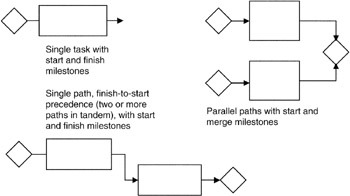
Figure 7-1: Schedule Building Blocks.
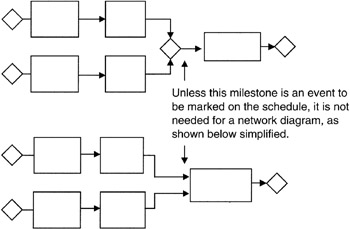
Figure 7-2: Milestone Simplifications.
There are certain characteristics that are applied to each schedule task, represented by a rectangle in our network building blocks. These task characteristics are:
- Every task has a specific beginning and a specific ending, thereby allowing for a specific duration (ending date minus beginning date) measured in some unit of time (for instance, hours, days, weeks, or months). Rarely would a schedule task be shown in years because the year is too coarse a measure for good project planning.
- Every task has some effort applied to it. Effort is measured in the hours spent by a "full-time equivalent" (FTE) working on the task. By example, if the effort on a task is 50 hours, and a FTE is 40 hours, then there is 1.25 FTE applied to the task. If the task duration is 25 hours, then the 50 hours of effort must be accomplished in 25 hours of calendar time, requiring 2.5 FTE. Thus, we have the following equations:
- FTE applied to task = (Effort/Duration) * (Effort/Hours per FTE)
- FTE applied to task = (50/25) * (50/40) = 2,500/1,000 = 2.5
- Every task has not only a specific beginning or ending, but also each task as an "earliest" or "latest" beginning or ending. The idea of earliest and latest leads to the ideas of float and critical path, which will be discussed in detail subsequently. Suffice it to say that the difference in "earliest" and "latest" is "float" and that tasks on the critical path have a float of precisely 0.
Estimating Duration and Effort
We can easily see that the significant metrics in every schedule network are the task durations and the task efforts. These two metrics drive almost all of the calculations, except where paths merge. We address the merge points in subsequent paragraphs. Now as a practical matter, when doing networks for some tasks it is more obvious and easier to apply the estimating ideas discussed in other chapters to the effort and let the duration be dependent on the effort and the number of FTE that can be applied. In other situations just the opposite is true: you have an idea of duration and FTE and the effort simply is derived by applying the equations we described above.
Most network software tools allow for setting defaults for effort-driven or duration-driven attributes for the whole project, or these attributes can be set task by task. For a very complex schedule, setting effort-driven or duration-driven attributes task by task can be very tedious indeed. Perhaps the best practical advice that can be given is to select the driver you are most comfortable with, and make selective adjustments on those tasks that are necessary. Consider this idea however: duration estimating ties your network directly to your program milestones. When a duration-driven network is developed, the ending dates or overall length of the network will fall on actual calendar dates. You will be able to see immediately if there is an inherent risk in the project network and the program milestones.
Perhaps the most important concept is the danger of using single-point estimates in durations and efforts. The PERT network was the first network system to recognize that the expected value is the best single estimate in the face of uncertainty, and therefore the expected value of the duration should be the number used in network calculations. The BETA distribution was selected for the PERT chart system and the two variables "alpha" and "beta" were picked to form a BETA curve with the asymmetry emphasizing the most pessimistic value. [1] Although the critical path method (CPM) to be discussed below started out using single-point estimates, in point of fact more often than not a three-point estimate is made, sometimes using the BETA curve and sometimes using the Triangular distribution. In effect, using three-point estimates in the CPM network makes such a CPM diagram little different from the PERT diagram.
[1]More information on the BETA "alpha" and "beta" parameters is provided in Chapter 2.
The Critical Path Method
One of the most common outcomes of the schedule network is the identification of one or more critical paths. Right at this point, let us say that the critical path, and in fact there may be more than one critical path through the network, may not be the most important path for purposes of business value or functionality. However, the critical path establishes the length of the network and therefore sets the overall duration of the project. If there is any schedule acceleration or delay along the critical path, then the project will finish earlier or later, respectively.
As a practical example of the difference between paths that are critical and functionally important, the author was once associated with a project to build an Intelsat ground station. The business value of the ground station was obviously to be able to communicate effectively with the Intelsat system and then make connectivity to the terrestrial communications system. However, the critical path on the project network schedule was the installation and operation of a voice intercom between the antenna pedestal and the ground communications control facility. The vendor selected for this intercom capability in effect set the critical path, though I am sure that all would agree that the intercom was not the most important functionality of the system. Nevertheless, the project was not complete until the intercom was delivered; any delay by the vendor (there was none) was a delay on the whole project.
Some Characteristics of the Critical Path
We have so far described the critical path as the longest path through the network. This is true and it is one of the clearest and most defining characteristics of the critical path.
A second idea is that there is no float or slack along the critical path. Having no float or slack means that if there is any change in durations along the critical path, then the overall schedule will be longer or shorter. In effect, such a characteristic means there is no schedule "reserve" that can isolate vagaries of the project with the fixed business milestones. In point of fact, almost no project is planned in this manner and the project manager usually plans a reserve task of time but not performance. We will see in our discussion of the "critical chain" concept that this reserve task is called a "buffer" and is managed solely by the project manager. Figure 7-3 illustrates this idea. For purposes of identifying and calculating the critical path, we will ignore the reserve task.
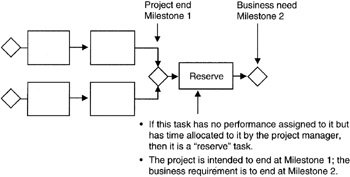
Figure 7-3: Reserve Task in Network.
A third idea is that there can be more than one critical path through the network. A change in duration on any one of the critical paths will change the project completion date, ignoring any reserve task.
Another notion is that of the "near-critical path." A near-critical path(s) is one or more paths that are not critical at the outset of the project, but could become critical. A path could become critical because the probabilistic outcomes of durations on one of these paths become longer than the identified critical path. Another possibility is that the critical path becomes shorter due to improved performance of its tasks and one of the "near-critical" paths is "promoted" to being the critical path. Such a set of events happens often in projects. Many project software tools have the capability of not only identifying and reporting on the near-critical path, but also calculating the probability that the path will become critical. Moreover, it is often possible to set a threshold so that the project manager sees only those paths on the report that exceed a set probability of becoming critical. In addition, it is possible to identify new paths that come onto the report or old paths that drop off the report because of ongoing performance during the course of the project.
Lastly, if there is only one connected path through the network, then there is only one critical path and that path is it; correspondingly, if the project is planned in such a way that no single path connects all the way through, then there is no critical path. As curious as the latter may seem, a network without a connecting path all the way through is a common occurrence in project planning. Why? It is a matter of having dependencies that are not defined in the network. Undefined dependencies are ghost dependencies. An early set of tasks does not connect to or drive a later set of tasks. The later set of tasks begins on the basis of a trigger from outside the project, or a trigger is not defined in the early tasks. Thus the latter tasks appear to begin at a milestone for which there is no dependency on the earlier tasks. In reality, such a network is really two projects and it should be handled as such. If addressed as two projects, then each will have a critical path. The overall length of the program (multiple projects) will depend on the two projects individually and the ghost task that connects one to the other. Such a situation is shown in Figure 7-4.
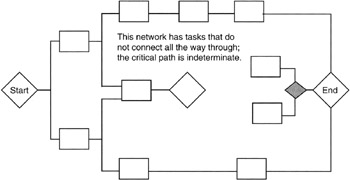
Figure 7-4: One Network as Two.
Calculating the Critical Path
Calculating the critical path is the most quantitatively intensive schedule management task to be done, perhaps more complicated than "resource leveling" and the calculation of merge points. Though intensive, critical path calculations are not hard to do, but on a practical basis critical path calculations are best left to schedule network software tools. The calculation steps are as follows:
- For each path in the network that connects all the way through, and in our examples we will employ only networks that do have paths that connect through, calculate the so-called "forward path" by calculating the path length using the earliest start dates.
- Then for each path in the network, work in the opposite direction, using latest finish dates, and calculate the "backward path."
- One or more paths calculated this way would have equal lengths, forward and backward. These are the critical paths. All other paths will have unequal forward and backward lengths. These paths are not critical.
- The amount of forward-backward inequality in any path is the float or slack in the path. Overall, this path, or any one task on this path, can slip by the amount of the forward-backward inequality and not be more than critical and therefore not delay the project.
Calculating the Forward Path
Figure 7-5 shows a simple network with the forward path calculation.
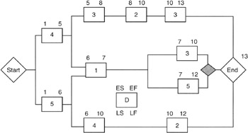
Figure 7-5: Forward Path Calculation.
We must adopt a notation convention. The tasks will be shown in rectangular boxes; the earliest start date will be on the upper left corner, and the earliest finish will be on the upper right corner. The corresponding lower corners will be used for latest start and finish dates, respectively. Duration will be shown in the rectangle.
In the forward path calculation, notice the use of the earliest start dates. The basic rule is simple:
Earliest start date + Duration = Earliest finish date
Now we have to be cognizant of the various precedence relationships such as finish-to-start and finish-to-finish, etc. All but finish-to-start greatly complicate the mathematics and are best left to scheduling software. Therefore, our example networks will all use finish-to-start relationships. There is no loss in generality since almost every network that has other than only finish-to-start relationships can be redrawn, employing more granularity, and become an all finish-to-start network.
Working in the forward path with finish-to-start relationships, the rule invoked is:
Earliest start of successor task = Latest of the early finish dates of all predecessors
The final milestone from the forward path analysis is an "earliest" finish milestone. Again, unless explicitly shown, any final management reserve task of unallocated reserve task is not shown for simplicity. If it were shown, it would move out, or shift right, the final milestone to align with the program milestones from the business side of the balance sheet.
Calculating the Backward Path
Now let's calculate the backward path. The very first question that arises is: "What is the date for the latest finish?" The backward path is calculated with the latest finish dates and all we have at this point is the earliest finish date. The answer is that if there is no final reserve task in the network, the latest finish date of the final milestone is taken to be the same as the earliest finish date calculated in the forward path. Having established a starting point for the backward path calculation, we then invoke the following equation:
Latest start = Latest finish - Duration
In calculating backward through the finish-to-start network, we use the earliest of the "latest start" dates of a successor task as the latest finish for a predecessor task. Figure 7-6 shows these calculations for our example network.
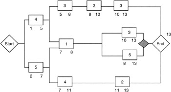
Figure 7-6: Backward Path Calculation.
Finding the Critical Tasks
Figure 7-7 shows the critical path calculation in one diagram for our example network. To find the critical path, it is a simple matter of identifying every task for which either of the following equations is true:
|
Earliest start (or finish) |
= |
Latest start (or finish) |
|
Earliest start (or finish) - Latest start (or finish) |
= |
0 = float or slack |
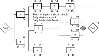
Figure 7-7: Critical Path Calculation.
Those tasks that obey the equations just given have zero slack or float. Such zero-float tasks are said to be critical and they form the one or more critical paths through the network.
The Central Limit Theorem Applied to Networks
Take notice that the critical path through the network always connects the beginning node or milestone and the ending node or milestone. The ending milestone can be thought of as the output milestone, and all the tasks in between are input to the final output milestone. Furthermore, if the project manager has used three-point estimates for the task durations, then the duration of any single task is a random variable best represented by the expected value of the task. [2] The total duration of the critical path from the input or beginning milestone to the output milestone, itself a 0-duration event, or the date assigned to the output milestone, represents the length of the overall schedule. The length of the overall schedule is a summation of random variables and is itself a random variable, L, of length:
L = Σ Di = (D1 + D2 + Di ...)
where Di are the durations of the tasks along the critical path.
We know from our discussion of the Central Limit Theorem that for a "large" number of durations in the sum the distribution of L will tend to be Normal regardless of the distributions of the individual tasks. This statement is precisely the case if all the distributions are the same for each task, but even if some are not, then the statement is so close to approximately true that it matters little to the project manager that L may not be exactly Normal distributed. Figure 7-8 illustrates this point.
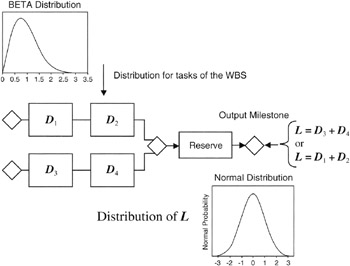
Figure 7-8: The Output Milestone Distribution.
Significance of Normal Distributed Output Milestone
The significance of the fact that the output milestone is approximately Normal distributed is not trivial. Here is why. Given the symmetry of the Normal curve, a Normal distributed output milestone means there is just as likely a possibility that the schedule will underrun (complete early) as overrun (complete late). Confronted with such a conclusion, most project managers would say: "No! The schedule is biased toward overrun." Such a reaction simply means that either the schedule is too short and the Normal output milestone is too aggressive, or the project manager has not thought objectively about the schedule risk.
Consider this conclusion about a Normal output milestone from another point of view. Without even considering what the distributions of the individual tasks on the WBS might be, whether BETA or Triangular or Normal or whatever, the project manager remains confident that the output milestone is Normal in its distribution! That is to say that there is a conclusion for every project, and it is the same conclusion for every project — the summation milestone of the critical path is approximately Normal. [3]
Calculating the Statistical Parameters of the Output Milestone
What the project manager does not know is the standard deviation or the variance of the Normal distribution. It is quite proper to ask of what real utility it is to know that the output milestone is Normal with an expected value (mean value) but have no other knowledge of the distribution. The answer is straightforward: either a schedule simulation can be run to determine the distribution parameters or, if there is no opportunity to individually estimate the tasks on the WBS, then the risk estimation effort can be moved to the output milestone as a practical matter.
At this point, there really is not an option about selecting the distribution since it is known to be Normal; if expected values have been used to compute the critical path, or some reasonable semblance of expected values has been used, then the mean of the output milestone is calculable. It then remains to make some risk assessment of the probable underrun. Usually we calculate the underrun distance from the mean as a most optimistic duration. Once done, this underrun estimate is identically the same as the distance from the expected value to the most pessimistic estimate. Such a conclusion is true because of the symmetry of the Normal distribution; underrun and overrun must be symmetrically located around the mean.
The last estimate to make is the estimate for the standard deviation. The standard deviation estimate is roughly one-sixth of the distance from the most optimistic duration estimate to the most pessimistic estimate.
Next, the Normal distribution for the outcome milestone is normalized to the standard Normal distribution. The standard Normal curve has mean = 0 and σ = 1. Once normalized, the project manager can apply the Normal distribution confidence curves to develop confidence intervals for communicating to the project sponsor.
Statistical Parameters of Other Program Milestones
The Central Limit Theorem is almost unlimited in its handiness to the project manager. Given that there is a "large number" of tasks leading up to any program or project milestone, and large is usually taken to be ten or more as a working estimate, then the distribution of that milestone is approximately Normal. The discussion of the output milestone applies in all respects, most importantly the statements about using the Normal confidence curves or tables.
Therefore, some good advice for every project manager is to obtain a handbook of numerical tables or learn to use the Normal function in any spreadsheet program that has statistical functions. Of course, every project manager learns the confidence figures for 1, 2, or 3 standard deviations: they are, respectively, 68.26, 95.46, and 98.76.
[2]Actually, whether or not the project manager proactively thinks about the random nature of the task durations and assigns a probability distribution to a task does not change the fact that the majority of tasks in projects (projects we define as one-time endeavors never done exactly the same way before) are risky and tasks have some randomness to their duration estimate. Therefore, the fact that the project manager does not or did not think about this randomness does not change the reality of the situation. Therefore, the conclusions cited in the text regarding the application of the Central Limit Theorem and the Law of Large Numbers are not invalidated by the fact that the project manager may not have gone to the effort to estimate the duration randomness.
[3]Strictly speaking, the Law of Large Numbers and the Central Limit Theorem are applicable to linear sums of durations. The critical path usually qualifies as a linear summation of durations. Merge points, fixed dates, and PDM relationships other than finish-to-start do not qualify.
Monte Carlo Simulation of the Network Performance
The arithmetic of finding expected value, standard deviation, and variance, at least to approximate values suitable and appropriate to project management, is not hard to do when working with the most common distributions we have described so far in this book. Anyone with reasonable proficiency in arithmetic can do it, and with a calculator or spreadsheet the math is really trivial. However, the manual methodology applied to a network of many tasks, or hundreds of tasks, or thousands, or even tens of thousands of tasks, is so tedious that the number of hand calculations is overwhelming and beyond practicality. Moreover, the usual approach when applying manual methods is to work only with the expected value of the distribution. The expected value is the best single number in the face of uncertainty, to be sure, but if the probability distribution has been estimated, then the distribution is a much more rich representation of the probable task performance than just the one statistic of the distribution called the expected value. Sensibly, whenever more information is available to the project manager, then it is appropriate to apply the more robust information set to the project planning and estimating activities.
If you can imagine that working only with the expected values is a tedious undertaking on a complex network, consider the idea of working with many points from each probability distribution from each task on the network. You immediately come to the conclusion that it is not possible to do such a thing manually. Thus, we look to computer-aided simulation to assist the project manager in evaluating the project network. One immediate advantage is that all the information about task performance represented by the probability distribution is available and usable in the computer simulation. There are many simulation possibilities, but one very popular one in common use and compatible with almost all scheduling programs and spreadsheets is the Monte Carlo simulation.
The Monte Carlo Simulation
The concept of operations behind the Monte Carlo simulation is quite simple: by using a Monte Carlo computer simulation program, [4] the network schedule is "run" or calculated many times, something we cannot usually do in real projects. Each time the schedule is run, a duration figure for each task is picked from the possible values within the pessimistic to optimistic range of the probability distribution for the task. Now each time the schedule is run, for any given task, the duration value that is picked will usually be different. Perhaps the first time the schedule is calculated, the most pessimistic duration is picked. The next time the schedule is run, perhaps the most likely duration is picked. In fact, over a large number of runs, wherein each run means calculating the schedule differently according to the probabilistic outcomes of the task durations, if we were to look at a report of the durations picked for a single task, it would appear that the values picked and their frequency of pick would look just like the probability distribution we assigned to the task. The most likely value would be picked the most and the most pessimistic or optimistic values would be picked least frequently. Table 7-1 shows such a report in histogram form. The histogram has a segregation or discrete quantification of duration values, and for each value there is a count of the number of times a duration value within the histogram quantification occurred.
|
"Standard" Normal Distribution of Outcome Milestone |
||
|---|---|---|
|
Normalized Outcome Value[a] (As Offset from the Expected Value) |
Histogram Value * 100[b] |
Cumulative Histogram * 100[b] (Confidence) |
|
-3 |
0.110796 |
0.110796 |
|
-2.75 |
0.227339 |
0.338135 |
|
-2.5 |
0.438207 |
0.776343 |
|
-2.25 |
0.793491 |
1.569834 |
|
-2 |
1.349774 |
2.919607 |
|
-1.75 |
2.156932 |
5.07654 |
|
-1.5 |
3.237939 |
8.314478 |
|
-1.25 |
4.566226 |
12.8807 |
|
-1 |
6.049266 |
18.92997 |
|
-0.75 |
7.528433 |
26.4584 |
|
-0.5 |
8.80163 |
35.26003 |
|
-0.25 |
9.6667 |
44.92673 |
|
0 |
9.973554 |
54.90029 |
|
0.25 |
9.6667 |
64.56699 |
|
0.5 |
8.80163 |
73.36862 |
|
0.75 |
7.528433 |
80.89705 |
|
1 |
6.049266 |
86.94632 |
|
1.25 |
4.566226 |
91.51254 |
|
1.5 |
3.237939 |
94.75048 |
|
1.75 |
2.156932 |
96.90741 |
|
2 |
1.349774 |
98.25719 |
|
2.25 |
0.793491 |
99.05068 |
|
2.5 |
0.438207 |
99.48888 |
|
2.75 |
0.227339 |
99.71622 |
|
3 |
0.110796 |
99.82702 |
|
[a]The outcome values lie along the horizontal axis of the probability distribution. For simplicity, the average value of the outcome (i.e., the mean or expected value) has been adjusted to 0 by subtracting the actual expected value from every outcome value: Adjusted outcomes = Actual outcomes - Expected value. After adjusting for the mean, the adjusted outcomes are then "normalized" to the standard deviation by dividing the adjusted outcomes by the standard deviation: Normalized outcomes = Adjusted outcomes/σ. After adjusting for the mean and normalizing to the standard deviation, we now have the "standard" Normal distribution. [b]The histogram value is the product of the horizontal value (outcome) times the vertical value (probability); the cumulative histogram, or cumulative probability, is the confidence that a outcome value, or a lesser value, will occur: Confidence = Probability outcome ≤ Outcome value. For better viewing, the cell area and the cumulative area have been multiplied by 100 to remove leading zeroes. The actual values are found by dividing the values shown by 100. |
||
Monte Carlo Simulation Parameters
The project manager gets to control many aspects of the Monte Carlo simulation. Such control gives the project manager a fair amount of flexibility to obtain the analysis desired. A few of the parameters usually under project manager control follow. The software package actually used will be the real control of these parameters, but typically:
- The distribution applied to each task, a group of tasks, or "globally" to the whole network can be picked from a list of choices.
- The distribution parameters can be specified, such as pessimistic and optimistic values, either in absolute value or as a percentage of the most likely value that is also specified.
- The task or milestone (one or more) that is going to be the "outcome" of the analysis can be picked.
- The number of runs can be picked. It is usually hard to obtain good results without at least 100 independent runs of the schedule. By independent we mean that all initial conditions are reset and there is no memory of results from one run to the next. For larger and more complex networks, running the schedule 100 times may take some number of minutes, especially if the computer is not optimized for such simulations. Better results are obtained with 1,000 or more runs. However, there is a practical trade-off regarding analysis time and computer resources. This trade-off is up to the project manager to handle and manage.
Monte Carlo Simulation Outcomes
At the outcome task of the simulation, the usual simulation products are graphical, tabular, and often presented as reports. Figure 7-9 shows typical data, including a "critical path and near-critical analysis" on paths that might be in the example network. The usual analysis products from a Monte Carlo simulation might include:
- A probability density distribution, with absolute values of outcome value and a vertical dimension scaled to meet the requirement that the sum of all probabilities equals 1
- A cumulative probability distribution, the so-called "S" curve, again scaled from 0 to 1 or 0 to 100% on the vertical axis and the value outcomes on the horizontal axis
- Other statistical parameters, such as mean and standard deviation
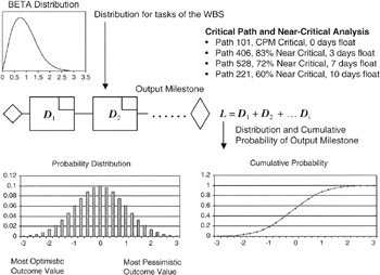
Figure 7-9: Monte Carlo Outcomes.
The Near Critical Path
Identification of near-critical paths that have a reasonable probability of becoming critical is a key outcome of Monte Carlo simulation. For many project managers, the near-critical path identification is perhaps the most important outcome. In fact, during the course of the Monte Carlo simulation, depending on the distributions applied to the critical tasks and the distributions applied to other paths, there will be many runs, perhaps very many runs, where the critical path identified by straightforward CPM calculations will not in fact be critical. Some other path, on a probabilistic basis, is critical for that particular run. Most Monte Carlo packages optimized for schedule applications keep careful record of all the paths that are, or become, critical during a session of runs. Appropriate reports are usually available.
Project managers can usually specify a threshold for reporting the near-critical paths. For example, perhaps the report contains only information about paths that have a 70% confidence, or higher, of becoming critical. Setting the threshold helps to separate the paths that are nearly critical and should be on a "watch list" along with the CPM-calculated critical path. If the schedule network is complex, such threshold reporting goes a long way in conserving valuable management time.
Convergence of Parameters in the Simulation
During the course of the session of 100 or more runs of the schedule, you may be able to observe the "convergence" of some of the statistical parameters to their final values. For instance, the expected value or standard deviation of the selected "outcome" task is going to change rapidly from the very first run to subsequent runs as more data are accumulated about the outcome distribution. After a point, if the parameter is being displayed, the project manager may well be able to see when convergence to the final value is "close enough." Such an observation offers the opportunity to stop the simulation manually when convergence is obtained. If the computer program does not offer such a real-time observation, there is usually some type of report that provides figures of merit about how well converged the reported parameters are to a final value.
There is no magic formula that specifies how close to the final value the statistical parameters like expected value, standard deviation, or variance should be for use in projects. Project managers get to be their own judge about such matters. Some trial and error may be required before a project manager is comfortable with final results.
Fixed Dates and Multiple Precedences in Monte Carlo Simulations
Fixed dates interfere with the Monte Carlo simulation by truncating the possible durations of tasks to fixed lengths or inhibiting the natural "shift-right" nature of merge points as discussed in the next section. Before running a simulation, the general rule of thumb is to go through your schedule and remove all fixed dates, then replace them with finish-to-start dependencies of project outcomes.
The same is usually said for precedences other than finish-to-start: redefine all precedences to finish-to-start before running the simulation. Many Monte Carlo results may be strange or even incorrect, depending on the sophistication of the package, if there are other than finish-to-start dependencies in the schedule. Again, the general rule of thumb is to go through your schedule and remove all relationships other than finish-to-start and replace them with an alternative network architecture of all finish-to-start dependencies of project outcomes. Although objectionable at first, the author has found that few networks really require other than finish-to-start relationships if the proper granularity of planning is done to identify all the points for finish-to-start, which obviates the need to use the other relationships.
[4]There are many PC and larger system software packages that will run a Monte Carlo simulation on a data set. In this chapter, our focus is on the network schedule, so the easiest approach is to obtain a package that "adds in" or integrates with your scheduling software. Of course, Monte Carlo simulation is not restricted to just schedule analysis. Any set of distributions can be analyzed in this way. For instance, the cost data from the WBS whereon each cost account has a probability distribution are candidates for Monte Carlo simulation. For cost analysis, an add-in to a spreadsheet or a statistical programs package would be ideal for running a Monte Carlo analysis of a cost data set.
Architecture Weaknesses in Schedule Logic
One of the problems facing project managers when constructing the logic of their project is avoiding inherently weak architectures in the schedule network. Certainly from the point of view of risk management, avoidance is a key strategy and well applied when developing the logic of the project. In this section we will address two architectural weaknesses that lend themselves to quantitative analysis: the merge point of parallel paths and the "long" task.
Merge Points in Network Logic
By merge point we simply mean a point in the logic where a milestone has two or more predecessors, each with the same finish date. Illustrations of network building blocks shown earlier in this chapter illustrate simple parallel paths joining at a milestone. Such a construction is exactly what we are talking about. Obviously, for all project managers such a logic situation occurs frequently and is really unavoidable entirely; the idea is to avoid as many merging points as possible.
Here is the problem in a nutshell. Let us assume that each of the merging paths is independent. By independent we mean that the performance along one path is not dependent on the performance along the other path. We must be careful here. If there are shared resources between the two paths that are in conflict, whether project staff, special tools, facilities, or other, then the paths are truly not independent. But assuming independence, there is a probability that path A will finish on the milestone date, p(A on time) = p(A), and there is a probability that path B will finish on the milestone date, p(B on time) = p(B). Now, the probability that the milestone into which each of the two paths merge will be achieved on time is the probability that both paths will finish on time. We know from the math of probabilities and from Bayes' Theorem that if A and B are independent, the probability of the milestone finishing on time is the product of the two probabilities:
p(Milestone on time) = p(A) * p(B)
Now it should be intuitively obvious what the problem is. Both p(A) and p(B) are numbers less than 1. Their product, p(A) * p(B), is even smaller, so the probability of meeting the milestone on time is less than the smallest probability of any of the joining paths. If there are more than two paths joining, the problem is that much greater. Figure 7-10 shows graphically the phenomenon we have been discussing.
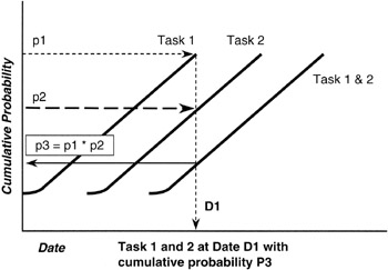
Figure 7-10: Merge Point Math.
Suppose that p(A) = 0.8 and p(B) = 0.7, both pretty high confidence figures. The joint probability of their product is quite simply: 0.8 * 0.7 = 0.56. Obviously, moving down from a confidence of 70% at the least for any single path to only 56% for the milestone is a real move and must be addressed by the project manager. To mitigate risk, the project manager would develop alternate schedule logic that does not require a merging of paths, or the milestone would be isolated with a buffer task.
We have mentioned "shift right" in the discussion of merge point. What does "shift right" refer to? Looking at Figure 7-10, we see that to raise the confidence of the milestone up to the least of the merging paths, in this case 70%, we are going to have to allow for more time. Such a conclusion is really straightforward: more time always raises the confidence in the schedule and provides for a higher probability of completion. But, of course, allowing more time is an extension, to the right, of the schedule. Extending the schedule to the right is the source of the term "shift right." The rule for project managers examining project logic is:
At every merge point of predecessor tasks, think "shift right."
Merging Dependent Paths
So far the discussion has been about the merging of independent paths. Setting the condition of independence certainly simplifies matters greatly. We know from our study of multiple random variables that if the random variables are not independent, then there is a covariance between them and a degree of correlation. We also know that if one path outcome is conditioned on the other path's outcome, then we must invoke Bayes' Theorem to handle the conditions.
p(A on time AND B on time) = p(A on time given B is on time) * p(B is on time)
We see right away on the right side of the equation that the "probability of A on time given B on time" is made smaller by the multiplication of the probability of "B on time." From what we have already discussed, making "probability of A on time given B on time" smaller is a shift right of the schedule. The exact amount is more difficult to estimate because of having to estimate "probability of A on time given B on time," but the heuristic is untouched: the milestone join of two paths, whether independent or not, will shift right. Only the degree of shift depends on the conditions between the paths.
Thinking of the milestone as an "outcome milestone," we can also approach this examination from the point of view of risk as represented by the variance of the outcome distribution. We may not know this distribution outright, although by the discussion that follows we might assume that it is somewhat Normal. In any event, if the two paths are not independent, what can we say about the variance of the outcome distribution at this point? Will it be larger or smaller?
We reason as follows: The outcome performance of the milestone is a combined effect of all the paths joining. If we look at the expected value of the two paths joining, and the paths are independent, then we know that:
E(A and B) = E(A) * E(B), paths independent
But if the paths are not independent, then the covariance between them comes into play:
E(A and B) = E(A) * E(B) + Cov(A and B)
where paths A and B are not independent.
The equation for the paths not independent tells us that the expected value may be larger (longer) or smaller (shorter) depending on the covariance. The covariance will be positive — that is, the outcome will be larger (the expected value of the outcome at the milestone is longer or shifted right) — if both paths move in the same direction together. This is often the case in projects because of the causes within the project that tend to create dependence between paths. The chief cause is shared resources, whether the shared resource is key staff, special tools or environments, or other unique and scarce resources. So the equation we are discussing is valuable heuristically even if we often do not have the information to evaluate it numerically. The heuristic most interesting to project managers is:
Parallel paths that become correlated by sharing resources stretch the schedule!
The observation that sharing resources will stretch the schedule is not news to most project managers. Either through experience or exposure to the various rules of thumb of project management, such a phenomenon is generally known. What we have done is given the rule of thumb a statistical foundation and given the project manager the opportunity, by means of the formula, to figure out the actual numerical impact. However, perhaps the most important way to make use of this discussion is by interpreting results from a Monte Carlo simulation. When running the Monte Carlo simulation, the effects of merge points and shift right will be very apparent. This discussion provides the framework to understand and interpret the results provided.
Resource Leveling Quantitative Effects
Resource leveling refers to the planning methodology in which scarce resources, typically staff with special skills (but also special equipment, facilities, and environments), are allocated to tasks where there is otherwise conflict for the resource. The situation we are addressing naturally arises out of multiple planners who each require a resource and plan for its use, only to find in the summation of the schedule network that certain resources are oversubscribed: there is simply too much demand for supply.
The first and most obvious solution is to increase supply. Sometimes increasing supply can work in the case of certain staff resources that can be augmented by contractors or temporary workers, and certain facilities or environments might likewise be outsourced to suppliers. However, the problem for quantitative analysis is the case where supply cannot be increased, demand cannot be reduced, and it is not possible physically to oversubscribe the resource. Some have said this is like the case of someone wondering if "nine women could have a baby in one month." It is also not unlike the situation described by Fredrick Brooks in his classic book, The Mythical Man-Month, [5] wherein he states affirmatively that the thought that a simple interchange of resources, like time and staff, is possible on complex projects is a myth! Interestingly enough, Brooks also states what he calls "Brooks Law":
Adding additional resources (increasing supply) to a late project only makes it later! [6]
For purposes of this book, we will limit our discussion of resource leveling to simply assigning resources in the most advantageous manner to affect the project in the least way possible. Several rules of thumb have been developed in this regard. The most prominent is perhaps: "assign resources to the critical path to ensure it is not resource starved, and then assign the remaining resources to the near-critical paths in descending order of risk." Certainly this is a sensible approach. Starving the critical path would seem to build in a schedule slip right away. Actually, however, others argue that in the face of scarce resources, the identification of the true critical path is obscured by the resource conflict.
Recall our discussion earlier about correlating or creating a dependency among otherwise independent paths. Resource leveling is exactly that. Most scheduling software has a resource leveling algorithm built in, and you can also buy add-in software to popular scheduling software that has more elaborate and more efficient algorithms. However, in the final analysis, creating a resource dependency among tasks almost certainly sets up a positive covariance between the paths. Recall that by positive covariance we mean that both path performances move in the same direction. If a scarce resource is delayed or retained on one path beyond its planned time, then surely it will have a similar impact on any other task it is assigned to, creating a situation of positive covariance.
Figure 7-11 and Figure 7-12 show a simple example. In Figure 7-11, we see a simple plan consisting of four tasks and two resources. Following the rule of thumb, we staff the critical path first and find that the schedule has lengthened as predicted by the positive covariance. In Figure 7-12, we see an alternate resource allocation plan, one in which we apparently do not start with the critical path, and indeed the overall network schedule is optimally shorter than first planned as shown in Figure 7-11. However, there is no combination of the two resources and the four tasks that is as short as if there were complete independence between tasks. Statistically speaking we would say that there is no case where the covariance can be zero in the given combination of tasks and resources.
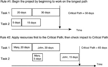
Figure 7-11: Resource Leveling Plan.
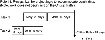
Figure 7-12: Resource Leveling Optimized.
Long Tasks
Another problem common to schedule network architecture is the so-called long task. What is "long" in this context? There is no exact answer, though there are many rules of thumb, heuristics. Many companies and some customers have built into their project methodology specific figures for task length that are not to be exceeded when planning a project unless a waiver is granted by the project manager. Some common heuristics of "short" tasks are 80 to 120 hours of FTE time or perhaps 10 to 14 days of calendar time. You can see by these figures that a long task is one measured in several weeks or many staff hours.
What is the problem with the long task from the quantitative methods point of view? Intuitively, the longer the task, the more likely something untoward will go wrong. As a matter of confidence in the long task, allowing for more possibilities to go wrong has to reduce the confidence in the task. Can we show this intuitive idea simply with statistics? Yes; let us take a look at the project shown in Figure 7-13.
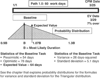
Figure 7-13: Long Task Baseline.
In Figure 7-13 we see a project consisting of only one task, and it is a long task. We have assigned a degree of risk to this long task by saying that the duration estimate is represented by a Triangular distribution with parameters as shown in the figure. We apply the equations we learned about expected value and variance and compute not only the variance and expected value but the standard deviation as well. It is handy to have the standard deviation because it is dimensioned the same as the expected value. Thus if the expected value is measured in days, then so will the standard deviation be. Unfortunately, the variance will be measured in days-squared with no physical meaning. Therefore the variance becomes a figure of merit wherein smaller is better.
The question at hand is whether we can achieve improvement in the schedule confidence by breaking up the long task into a waterfall of tandem but shorter tasks. Our intuition guided by the Law of Large Numbers tells us we are on the right track. If it is possible for the project manager and the WBS work package managers to redesign the work so that the WBS work package can be subdivided into smaller but tandem tasks, then even though each task has a dependency on its immediate predecessor, our feeling is that with the additional planning knowledge that leads to breaking up the long task should come higher confidence that we have it estimated more correctly.
For simplicity, let's apply the Triangular distribution to each of the shorter tasks and also apply the same overall assumptions of pessimism and optimism. You can work some examples to show that there is no loss of generality in the final conclusion. We now recompute the expected value of the overall schedule and the variance and standard deviation of the output milestone. We see a result predicted by the Law of Large Numbers as illustrated in Figure 7-14. The expected value of the population is the expected value of the outcome (summation) milestone. Our additional planning knowledge does not change the expected value. However, note the improvement in the variance and the standard deviation; both have improved. Not coincidently, the (sample) variance has improved, compared to the population variance, by 1/N, where N is the number of tasks into which we subdivided the longer task, and the standard deviation has improved by 1/√N. We need only look back to our discussion of the sample variance to see exactly from where these results come.
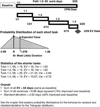
Figure 7-14: Shorter Tasks Project.
[5]Brooks, Fredrick P., The Mythical Man-Month, Addison Wesley Longman, Inc., Reading, MA, 1995, p. 16.
[6]Brooks, Fredrick P., The Mythical Man-Month, Addison Wesley Longman, Inc., Reading, MA, 1995, p. 25.
Rolling Wave Planning
In Chapter 6 (in the discussion about cost accounting), we noted that it is not often possible to foresee the future activities in a project with consistent detail over the entire period of the project. Therefore, planning is often done in "waves" or stages, with the activities in the near term planned in detail and the activities in the longer distance of time left for future detail planning. There may in fact be several planning waves, particularly if the precise approach or resource requirement is dependent or conditioned on the near-term activities. Such a planning approach is commonly called rolling wave planning.
Rolling Wave Characteristics
The fact is that the distinguishing characteristic of the planning done now for a future wave is that both cost accounts and network tasks are "long" (or "large") compared to their near-term counterparts. We have already discussed the long task in this discussion. Project managers can substitute the words "large cost account" for "long task" and all of the statistical discussions apply, except that the principles and techniques are applied to the cost accounts on the WBS and not to the network schedule.
Monte Carlo Effects in the Rolling Wave
Whether you are doing a Monte Carlo analysis on the WBS cost or on the network schedule, the longer tasks and larger work packages have greater variances. The summation of the schedule at its outcome milestone or the summation of the WBS cost at the top of the WBS will be a Normal distributed outcome regardless of the rolling waves. However, the Monte Carlo simulation will show you what you intuitively know: the longer task and larger cost accounts, with their comparatively larger variances, will increase the standard deviation of the Normal distribution, flatten its curve, and stretch its tails.
As the subsequent waves come and more details are added, the overall variances will decrease and the Normal distribution of the outcome variable, whether cost or schedule, will become more sharply defined, the tails will be less extreme, and the standard deviation (which provides the project manager entree to the confidence tables) will be more meaningful.
The Critical Chain
There is a body of knowledge in schedule and resource planning that has grown since 1997 when Eliyahu M. Goldratt wrote Critical Chain, [7] arguably one of the most significant books in project management. In this book, written like a novel rather than a textbook, Goldratt applies to project management some business theories he developed earlier for managing in a production operation or manufacturing environment. Those theories are collectively called the Theory of Constraints. As applied to project management, Goldratt asserts that the problem in modern project management is ineffective management of the critical path, because the resources necessary to ensure a successful critical path are unwittingly or deliberately scattered and hidden in the project.
The Theory of Constraints
In the Theory of Constraints, described in another Goldratt business novel, The Goal, [8] the idea put forward is that in any systemic chain of operations, there is always one operation that constrains or limits the throughput of the entire chain. Throughput is generally thought of as the value-add product produced by the operation that has value to the customer. If the chain of operations is stable and not subject to too many random errors, then the constraint is stable and identifiable; in other words, the constraint is not situational and does not move around from one job session, batch, or run to the next.
To optimize the operation, Goldratt recommends that if the capacity of the constraint cannot be increased, or the constraint cannot be removed by process redesign, then all activities ahead of the constraint should be operated in such a manner that the constraint is never starved. Also, activities ahead of the constraint should never work harder, faster, or more productively than the minimum necessary to keep the constraint from being starved. Some may recognize this latter point as a plank from the "just-in-time" supply chain mantra, and in fact that is not a bad way to look at it, but Goldratt's main point was to identify and manage the constraint optimally.
From Theory of Constraints to Critical Chain
When Goldratt carried his ideas to project management, he identified the project constraint as the critical path. By this association, what Goldratt means is that the project is constrained to a certain duration, and that constrained duration cannot be made shorter. The consequence of the critical path is that constrained throughput (valuable deliverables to the project sponsor) cannot be increased, and indeed throughput is endangered if the critical path cannot be properly managed.
Goldratt made several recommendations in his book Critical Chain, but the most prominent are:
- The tasks on the critical path do indeed require statistical distributions to estimate the range of pessimism to optimism. But, unlike PERT [9] or CPM, [10] Goldratt insists that the median value, the 50% confidence level, be used. Using the median value, the so-called 50-50 point, means that there is equal likelihood that the task will underrun as overrun.
- All task activity in the project schedule network that is not on the critical path should be made subordinate to the demands of the critical path.
- There should be "buffers" built into any path that joins the critical path. A buffer is a task of nonzero duration but has no performance requirement. In effect, buffer is another word for reserve. However, Goldratt recommends that these buffers be deliberately planned into the project.
- By using the median figure for each task on the critical path, Goldratt recognizes that the median figure is generally more optimistic than the CPM most likely estimate and is often more optimistic than the expected value. Goldratt recommends that the project manager "gather up" the excess pessimism and put it all into a "project buffer" at the end of the network schedule to protect the critical path.
We have already discussed Goldratt's point about a project buffer in our earlier discussion about how to represent the project schedule risk as calculated on the network with the project sponsor's business value dates as set in the program milestones. We did not call it a buffer in that discussion, but for all intents and purposes, that is what it is. Figure 7-15 illustrates the placement of buffers in critical chain planning.
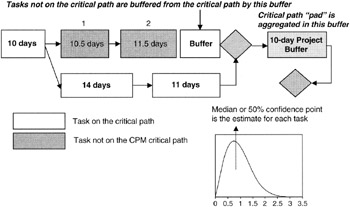
Figure 7-15: Critical Chain Buffers.
The critical chain ideas are somewhat controversial in the project management community, though there is no lack of derivative texts, papers, projects with lessons learned, and practitioners that are critical chain promoters. The controversy arises out of the following points:
- Can project teams really be trained to estimate with the median value? If so, then the critical chain by Goldratt's description can be established.
- Can team leaders set up schedule buffers by taking away schedule "pad" from cost account managers, or does the concept of buffers simply lead to "pad" on top of "pad"? To the extent that all cost account managers and team leaders will manage to the same set of principles, the critical chain can be established.
[7]Goldratt, Eliyahu M., Critical Chain, North River Press, Great Barrington, MA, 1997.
[8]Goldratt, Eliyahu M. and Cox, Jeff, The Goal, North River Press, Great Barrington, MA, 1985.
[9]PERT uses the BETA distribution and requires that the expected value be used.
[10]CPM traditionally uses a single-point estimate and, more often than not, the single estimate used is the "most likely" outcome and not the expected value.
Summary of Important Points
Table 7-2 provides the highlights of this chapter.
|
Point of Discussion |
Summary of Ideas Presented |
|---|---|
|
Quantitative time management |
|
|
Critical path |
|
|
Central Limit Theorem and schedules |
|
|
Monte Carlo simulation |
|
|
Architecture weaknesses |
|
|
Critical chain |
|
References
1. Brooks, Fredrick P., The Mythical Man-Month, Addison Wesley Longman, Inc., Reading, MA, 1995, p. 16.
2. Brooks, Fredrick P., The Mythical Man-Month, Addison Wesley Longman, Inc., Reading, MA, 1995, p. 25.
3. Goldratt, Eliyahu M., Critical Chain, North River Press, Great Barrington, MA, 1997.
4. Goldratt, Eliyahu M. and Cox, Jeff, The Goal, North River Press, Great Barrington, MA, 1985.
Preface
- Project Value: The Source of all Quantitative Measures
- Introduction to Probability and Statistics for Projects
- Organizing and Estimating the Work
- Making Quantitative Decisions
- Risk-Adjusted Financial Management
- Expense Accounting and Earned Value
- Quantitative Time Management
- Special Topics in Quantitative Management
- Quantitative Methods in Project Contracts
EAN: 2147483647
Pages: 97
